While the proliferation of cameras attached to mobile computers has been a boon for photography, there is much more that this can enable. Beyond simply capturing the outside world, the right software running on more powerful hardware can allow these computers to understand the things their cameras see.
This small bit of understanding can enable some truly powerful applications, such as barcode scanning, document recognition and imaging, translation of written words, real-time image stabilization, and augmented reality. As processing power, camera fidelity, and algorithms advance, this machine vision will be able to solve even more important problems.
Many people regard machine vision as a complex discipline, far outside the reach of everyday programmers. I don't believe that's the case. I created an open-source framework called GPUImage in large part because I wanted to explore high-performance machine vision and make it more accessible.
GPUs are ideally suited to operate on images and video because they are tuned to work on large collections of data in parallel, such as the pixels in an image or video frame. Depending on the operation, GPUs can process images hundreds or even thousands of times faster than CPUs can.
One of the things I learned while working on GPUImage is how even seemingly complex image processing operations can be built from smaller, simpler ones. I'd like to break down the components of some common machine vision processes, and show how these processes can be accelerated to run on modern GPUs.
Every operation analyzed here has a full implementation within GPUImage, and you can try each one yourself by grabbing the project and building the FilterShowcase sample application either for OS X or iOS. Additionally, all of these operations have CPU-based (and some GPU-accelerated) implementations within the OpenCV framework, which Engin Kurutepe talks about in his article within this issue.
Sobel Edge Detection
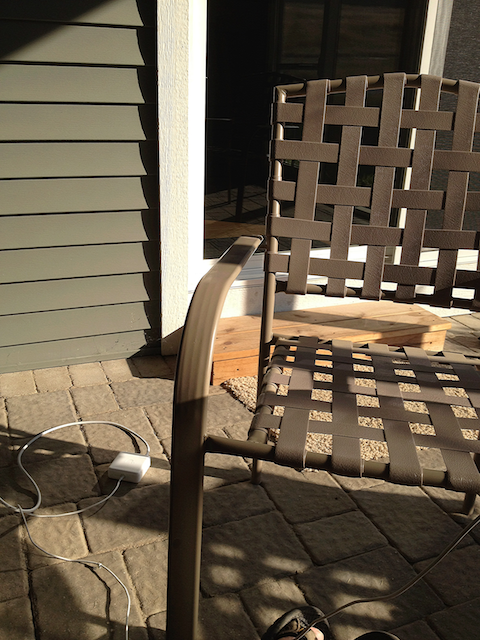
The first operation I'll describe may actually be used more frequently for cosmetic image effects than machine vision, but it's a good place to start. Sobel edge detection is a process where edges (sharp transitions from light to dark, or vice versa) are found within an image. 1 The strength of an edge around a pixel is reflected in how bright that pixel is in the processed image.
For example, let's see a scene before and after Sobel edge detection:
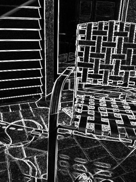
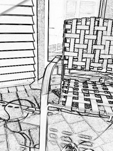
As I mentioned, this is often used for visual effects. If the colors of the above are inverted, with the strongest edges represented in black instead of white, we get an image that resembles a pencil sketch:
So how are these edges calculated? The first step in this process is a reduction of a color image to a luminance (grayscale) image. Janie Clayton explains how this is calculated in a fragment shader within her article, but basically the red, green, and blue components of each pixel are weighted and summed to arrive at a single value for how bright that pixel is.
Some video sources and cameras provide YUV-format images, rather than RGB. The YUV color format splits luminance information (Y) from chrominance (UV), so for these types of inputs, a color conversion step can be avoided. The luminance part of the image can be used directly.
Once an image is reduced to its luminance, the edge strength near a pixel is calculated by looking at a 3×3 array of neighboring pixels. An image processing calculation performed over a block of pixels involves what is called a convolution kernel. Convolution kernels consist of a matrix of weights that are multiplied with the values of the pixels surrounding a central pixel, with the sum of those weighted values determining the final pixel value.
These kernels are applied once per pixel across the entire image. The order in which pixels are processed doesn't matter, so a convolution across an image is an easy operation to parallelize. As a result, this can be greatly accelerated by running on a programmable GPU using fragment shaders. As described in Janie's article, fragment shaders are C-like programs that can be used by GPUs to perform incredibly fast image processing.
This is the horizontal kernel of the Sobel operator:
| −1 | 0 | +1 |
| −2 | 0 | +2 |
| −1 | 0 | +1 |
To apply this to a pixel, the luminance is read from each surrounding pixel. If the input image has been converted to grayscale, this can be sampled from any of the red, green, or blue color channels. The luminance of a particular surrounding pixel is multiplied by the corresponding weight from the above matrix and added to the total.
How this works to find an edge in a direction is that it looks for differences in luminance (brightness) on the left and right sides of a central pixel. If you have two equally bright pixels on the left and right of the center one (a smooth area in the image), the product of their intensities and the negative and positive weights will cancel out, and no edge will be detected. If there is a difference between the brightness of pixels on the left and right (an edge), one brightness will be subtracted from the other. The greater the difference, the stronger the edge measured.
The Sobel operator has two stages, the horizontal kernel being the first. A vertical kernel is applied at the same time, with the following matrix of weights:
| −1 | −2 | −1 |
| 0 | 0 | 0 |
| +1 | +2 | +1 |
The final weighted sum from each operator is tallied, and the square root of the sums of their squares is obtained. The squares are used because the values might be negative or positive, but we want their magnitude, not their sign. There's also a handy built-in GLSL function that does this for us.
That combined value is then used as the luminance for the final output image. Sharp transitions from light to dark (or vice versa) become bright pixels in the result, due to the Sobel kernels emphasizing differences between pixels on either side of the center.
There are slight variations to Sobel edge detection, such as Prewitt edge detection, 2 that use different weights for the horizontal and vertical kernels, but they rely on the same basic process.
As an example for how this can be implemented in code, the following is an OpenGL ES fragment shader that performs Sobel edge detection:
								precision mediump float;

varying vec2 textureCoordinate;
varying vec2 leftTextureCoordinate;
varying vec2 rightTextureCoordinate;

varying vec2 topTextureCoordinate;
varying vec2 topLeftTextureCoordinate;
varying vec2 topRightTextureCoordinate;

varying vec2 bottomTextureCoordinate;
varying vec2 bottomLeftTextureCoordinate;
varying vec2 bottomRightTextureCoordinate;

uniform sampler2D inputImageTexture;

void main()
{
   float bottomLeftIntensity = texture2D(inputImageTexture, bottomLeftTextureCoordinate).r;
   float topRightIntensity = texture2D(inputImageTexture, topRightTextureCoordinate).r;
   float topLeftIntensity = texture2D(inputImageTexture, topLeftTextureCoordinate).r;
   float bottomRightIntensity = texture2D(inputImageTexture, bottomRightTextureCoordinate).r;
   float leftIntensity = texture2D(inputImageTexture, leftTextureCoordinate).r;
   float rightIntensity = texture2D(inputImageTexture, rightTextureCoordinate).r;
   float bottomIntensity = texture2D(inputImageTexture, bottomTextureCoordinate).r;
   float topIntensity = texture2D(inputImageTexture, topTextureCoordinate).r;

   float h = -bottomLeftIntensity - 2.0 * leftIntensity - topLeftIntensity + bottomRightIntensity + 2.0 * rightIntensity + topRightIntensity;
   float v = -topLeftIntensity - 2.0 * topIntensity - topRightIntensity + bottomLeftIntensity + 2.0 * bottomIntensity + bottomRightIntensity;
   float mag = length(vec2(h, v));

   gl_FragColor = vec4(vec3(mag), 1.0);
}
The above shader has manual names for the pixels around the center one, passed in from a custom vertex shader, due to an optimization to reduce dependent texture reads on mobile devices. After these named pixels are sampled in a 3×3 grid, the horizontal and vertical Sobel kernels are applied using hand-coded calculations. The 0-weight entries are left out, in order to simplify these calculations. The GLSL length() function calculates a Pythagorean hypotenuse between the results of the horizontal and vertical kernels. That magnitude value is then copied into the red, green, and blue channels of the output pixel to produce a grayscale indication of edge strength.
Canny Edge Detection
Sobel edge detection can give you a good visual measure of edge strength in a scene, but it doesn't provide a yes/no indication of whether a pixel lies on an edge or not. For such a decision, you could apply a threshold of some sort, where pixels above a certain edge strength are considered to be part of an edge. However, this isn't ideal, because it tends to produce edges that are many pixels wide, and choosing an appropriate threshold can vary with the contents of an image.
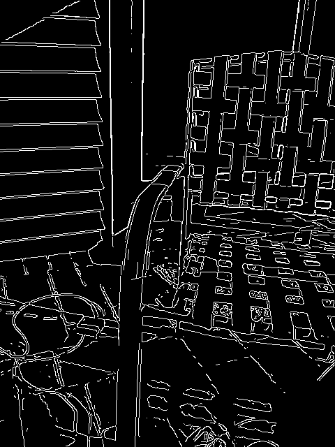
A more involved form of edge detection, called Canny edge detection, 3 might be what you want here. Canny edge detection can produce connected, single-pixel-wide edges of objects in a scene:
The Canny edge detection process consists of a sequence of steps. First, like with Sobel edge detection (and the other techniques we'll discuss), the image needs to be converted to luminance before edge detection is applied to it. Once a grayscale luminance image has been obtained, a slight Gaussian blur is used to reduce the effect of sensor noise on the edges being detected.
After the image has been prepared, the edge detection can be performed. The specific GPU-accelerated process used here was originally described by Ensor and Hall in "GPU-based Image Analysis on Mobile Devices." 4
First, both the edge strength at a given pixel and the direction of the edge gradient are determined. The edge gradient is the direction in which the greatest change in luminance is occurring. This is perpendicular to the direction the edge itself is running.
To find this, we use the Sobel kernel described in the previous section. The magnitude of the combined horizontal and vertical results gives the edge gradient strength, which is encoded in the red component of the output pixel. The horizontal and vertical Sobel results are then clamped to one of eight directions (corresponding to the eight pixels surrounding the central pixel), and the X component of that direction is encoded in the green component of the pixel. The Y component is placed into the blue component.
The shader used for this looks like the Sobel edge detection one above, only with the final calculation replaced with this code:
									vec2 gradientDirection;
	gradientDirection.x = -bottomLeftIntensity - 2.0 * leftIntensity - topLeftIntensity + bottomRightIntensity + 2.0 * rightIntensity + topRightIntensity;
	gradientDirection.y = -topLeftIntensity - 2.0 * topIntensity - topRightIntensity + bottomLeftIntensity + 2.0 * bottomIntensity + bottomRightIntensity;

	float gradientMagnitude = length(gradientDirection);
	vec2 normalizedDirection = normalize(gradientDirection);
	normalizedDirection = sign(normalizedDirection) * floor(abs(normalizedDirection) + 0.617316); // Offset by 1-sin(pi/8) to set to 0 if near axis, 1 if away
	normalizedDirection = (normalizedDirection + 1.0) * 0.5; // Place -1.0 - 1.0 within 0 - 1.0

	gl_FragColor = vec4(gradientMagnitude, normalizedDirection.x, normalizedDirection.y, 1.0);
To refine the Canny edges to be a single pixel wide, only the strongest parts of the edge are kept. For that, we need to find the local maximum of the edge gradient at each slice along its width.
This is where the gradient direction we calculated in the last step comes into play. For each pixel, we look at the nearest neighboring pixels both forward and backward along this length, and compare their calculated gradient strength (edge intensity). If the current pixel's gradient strength is greater than those of the ones forward and backward along the gradient, we keep that pixel. If the strength is less than either of the neighboring pixels, we reject that pixel and turn it to black.
A shader to do this appears as follows:
								precision mediump float;

varying highp vec2 textureCoordinate;

uniform sampler2D inputImageTexture;
uniform highp float texelWidth;
uniform highp float texelHeight;
uniform mediump float upperThreshold;
uniform mediump float lowerThreshold;

void main()
{
    vec3 currentGradientAndDirection = texture2D(inputImageTexture, textureCoordinate).rgb;
    vec2 gradientDirection = ((currentGradientAndDirection.gb * 2.0) - 1.0) * vec2(texelWidth, texelHeight);

    float firstSampledGradientMagnitude = texture2D(inputImageTexture, textureCoordinate + gradientDirection).r;
    float secondSampledGradientMagnitude = texture2D(inputImageTexture, textureCoordinate - gradientDirection).r;

    float multiplier = step(firstSampledGradientMagnitude, currentGradientAndDirection.r);
    multiplier = multiplier * step(secondSampledGradientMagnitude, currentGradientAndDirection.r);

    float thresholdCompliance = smoothstep(lowerThreshold, upperThreshold, currentGradientAndDirection.r);
    multiplier = multiplier * thresholdCompliance;

    gl_FragColor = vec4(multiplier, multiplier, multiplier, 1.0);
}
Here, texelWidth and texelHeight are the distances between neighboring pixels in the input texture, and lowerThreshold and upperThreshold set limits on the range of edge strengths we want to examine in this.
As a last step in the Canny edge detection process, pixel gaps in the edges are filled in to complete edges that might have had a few points failing the threshold or non-maximum suppression tests. This cleans up the edges and helps to make them continuous.
This last step looks at all the pixels around a central pixel. If the center was a strong pixel from the previous non-maximum suppression step, it remains a white pixel. If it was a completely suppressed pixel, it stays as a black pixel. For middling grey pixels, the neighborhood around them is evaluated. Each one touched by more than one white pixel becomes a white pixel. If not, it goes to black. This fills in the gaps in detected edges.
As you can tell, the Canny edge detection process is much more involved than Sobel edge detection, but it can yield nice, clean lines tracing around the edges of objects. This gives a good starting point for line detection, contour detection, or other image analysis, and can also be used to produce some interesting aesthetic effects.
Harris Corner Detection
While the previous edge detection techniques can extract some information about an image, the result is an image with visual clues about the locations of edges, not higher-level information about what is present in a scene. For that, we need algorithms that process the pixels within a scene and return more descriptive information about what is shown.
A popular starting point for object detection and matching is feature detection. Features are points of interest in a scene — locations that can be used to uniquely identify structures or objects. Corners are commonly used as features, due to the information contained in the pattern of abrupt changes in lighting and/or color around a corner.
One technique for detecting corners was proposed by Harris and Stephens in "A Combined Corner and Edge Detector." 5 This so-called Harris corner detector uses a multi-step process to identify corners within scenes.
As with the other processes we've talked about, the image is first reduced to luminance. The X and Y gradients around a pixel are determined using a Sobel, Prewitt, or related kernel, but they aren't combined to yield a total edge magnitude. Instead, the X gradient strength is passed along in the red color component, the Y gradient strength in the green color component, and the product of the X and Y gradient strengths in the blue color component.
A Gaussian blur is then applied to the result of that calculation. The values encoded in the red, green, and blue components are extracted from that blurred image and used to populate the variables of an equation for calculating the likelihood that a pixel is a corner point:
R = I x 2 × I y 2 − I xy × I xy − k × (I x 2 + I y 2 ) 2
Here, I x is the gradient intensity in the X direction (the red component in the blurred image), I y is the gradient intensity in Y (the green component), I xy is the product of these intensities (the blue component), k is a scaling factor for sensitivity, and R is the resulting "cornerness" of the pixel. Alternative implementations of this calculation have been proposed by Shi and Tomasi 6 and Noble, 7 but the results tend to be fairly similar.
Looking at this equation, you might think that the first two terms should cancel themselves out. That's where the Gaussian blur of the previous step matters. By blurring the X, Y, and product of X and Y values independently across several pixels, differences develop around corners and allow for them to be detected.
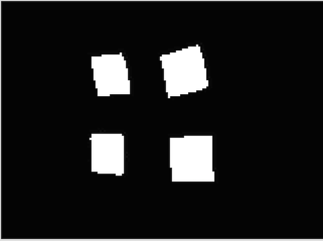
Here we start with a test image drawn from this question on the Signal Processing Stack Exchange site:
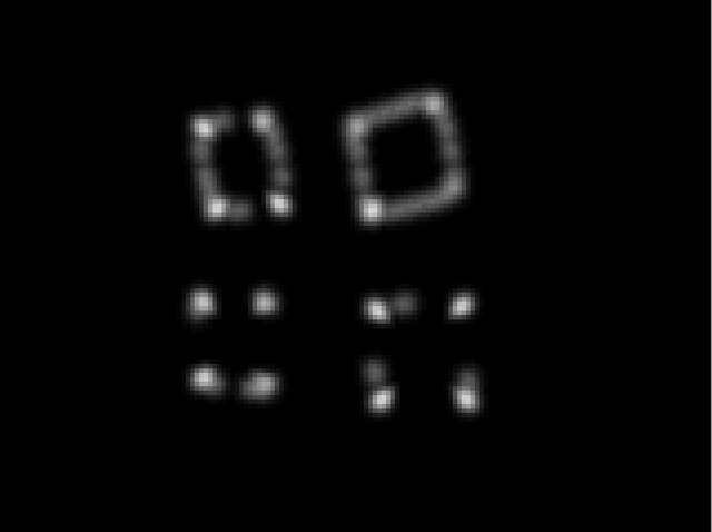
The resulting cornerness map from the above calculation looks something like this:
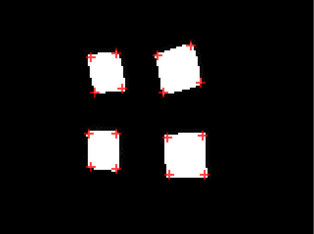
To find the exact location of corners within this map, we need to pick out local maxima (pixels of highest brightness in a region). A non-maximum suppression filter is used for this. Similar to what we did with the Canny edge detection, we now look at pixels surrounding a central one (starting at a one-pixel radius, but this can be expanded), and only keep a pixel if it is brighter than all of its neighbors. We turn it to black otherwise. This should leave behind only the brightest pixels in a general region, or those most likely to be corners.
From that, we now can read the image and see that any non-black pixel is a location of a corner:
I'm currently doing this point extraction stage on the CPU, which can be a bottleneck in the corner detection process, but it may be possible to accelerate this on the GPU using histogram pyramids. 8
The Harris corner detector is but one means of finding corners within a scene. Edward Rosten's FAST corner detector, as described in "Machine learning for high-speed corner detection," 9 is a higher-performance corner detector that may also outpace the Harris detector for GPU-bound feature detection.
Hough Transform Line Detection
Straight lines are another large-scale feature we might want to detect in a scene. Finding straight lines can be useful in applications ranging from document scanning to barcode reading. However, traditional means of detecting lines within a scene haven't been amenable to implementation on a GPU, particularly on mobile GPUs.
Many line detection processes are based on a Hough transform, which is a technique where points in a real-world, Cartesian coordinate space are converted to another coordinate space. Calculations are then performed in this alternate coordinate space and the results converted back into normal space to determine the location of lines or other features. Unfortunately, many of these proposed calculations aren't suited for being run on a GPU because they aren't sufficiently parallel in nature, and they require intense mathematical operations, like trigonometry functions, to be performed at each pixel.
In 2011, Dubská, et al. 10 11 proposed a much simpler, more elegant way of performing this coordinate space transformation and analysis — one that was ideally suited to being run on a GPU. Their process relies on a concept called parallel coordinate space, which sounds completely abstract, but I'll show how it's actually fairly simple to understand.
Let's take a line and pick three points within it:
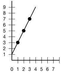
To transform this to parallel coordinate space, we'll draw three parallel vertical axes. On the center axis, we'll take the X components of our line points and draw points at 1, 2, and 3 steps up from zero. On the left axis, we'll take the Y components of our line points and draw points at 3, 5, and 7 steps up from zero. On the right axis, we'll do the same, only we'll make the Y values negative.
We'll then connect the Y component points to the corresponding X-coordinate component on the center axis. That creates a drawing like the following:
![]()
You'll notice that the three lines on the right intersect at a point. This point determines the slope and intercept of our line in real space. If we had a line that sloped downward, we'd have an intersection on the left half of this graph.
If we take the distance from the center axis and call that u (2 in this case), take the vertical distance from zero and call that v (1/3 in this case), and then label the width between our axes d (6, based on how I spaced the axes in this drawing), we can calculate slope and Y-intercept using the following equations:
slope = −1 + d/u
intercept = d × v/u
The slope is thus 2, and the Y-intercept 1, matching what we drew in our line above.
GPUs are excellent at this kind of simple, ordered line drawing, so this is an ideal means of performing line detection on the GPU.
The first step in detecting lines within a scene is finding the points that potentially indicate a line. We're looking for points on edges, and we want to minimize the number of points we're analyzing, so the previously described Canny edge detection is an excellent starting point.
After the edge detection, the edge points are read and used to draw lines in parallel coordinate space. Each edge point has two lines drawn for it, one between the center and left axes, and one between the center and right axes. We use an additive blending mode so that pixels where lines intersect get brighter and brighter. The points of greatest brightness in an area indicate lines.
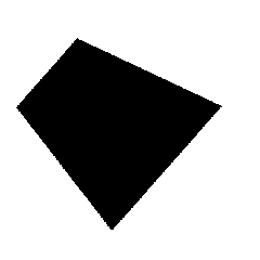
For example, we can start with this test image:
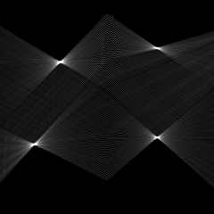
And this is what we get in parallel coordinate space (I've shifted the negative half upward to halve the Y space needed):
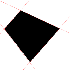
Those bright central points are where we detect lines. A non-maximum suppression filter is then used to find the local maxima and reduce everything else to black. From there, the points are converted back to line slopes and intercepts, yielding this result:
I should point out that the non-maximum suppression is one of the weaker points in the current implementation of this within GPUImage. It causes lines to be detected where there are none, or multiple lines to be detected near strong lines in a noisy scene.
As mentioned earlier, line detection has a number of interesting applications. One particular application this enables is one-dimensional barcode reading. An interesting aspect of this parallel coordinate transform is that parallel lines in real space will always appear as a series of vertically aligned dots in parallel coordinate space. This is true no matter the orientation of the parallel lines. That means that you could potentially detect standard 1D barcodes at any orientation or position by looking for a specific ordered spacing of vertical dots. This could be a huge benefit for blind users of mobile phone barcode scanners who cannot see the box or orientation they need to align barcodes within.
Personally, the geometric elegance of this line-drawing process is something I find fascinating and wanted to present to more developers.
Summary
These are but some of the many machine vision operations that have been developed in the last few decades, and only a small portion of the ones that can be adapted to work well on a GPU. I personally think there is exciting and groundbreaking work left to be done in this area, with important applications that can improve the way of life for many people. Hopefully, this has at least provided a brief introduction to the field of machine vision and shown that it's not as impenetrable as many developers believe.
-
I. Sobel. An Isotropic 3x3 Gradient Operator, Machine Vision for Three-Dimensional Scenes, Academic Press, 1990. ↩
-
J.M.S. Prewitt. Object Enhancement and Extraction, Picture processing and Psychopictorics, Academic Press, 1970. ↩
-
J. Canny. A Computational Approach To Edge Detection, IEEE Trans. Pattern Analysis and Machine Intelligence, 8(6):679–698, 1986. ↩
-
A. Ensor, S. Hall. GPU-based Image Analysis on Mobile Devices. Proceedings of Image and Vision Computing New Zealand 2011. ↩
-
C. Harris and M. Stephens. A Combined Corner and Edge Detector. Proc. Alvey Vision Conf., Univ. Manchester, pp. 147-151, 1988. ↩
-
J. Shi and C. Tomasi. Good features to track. Proceedings of the IEEE Conference on Computer Vision and Pattern Recognition, pages 593-600, June 1994. ↩
-
A. Noble. Descriptions of Image Surfaces. PhD thesis, Department of Engineering Science, Oxford University 1989, p45. ↩
-
G. Ziegler, A. Tevs, C. Theobalt, H.-P. Seidel. GPU Point List Generation through HistogramPyramids. Research Report, Max-Planck-Institut fur Informatik, 2006. ↩
-
E. Rosten and T. Drummond. Machine learning for high-speed corner detection. European Conference on Computer Vision 2006. ↩
-
M. Dubská, J. Havel, and A. Herout. Real-Time Detection of Lines using Parallel Coordinates and OpenGL. Proceedings of SCCG 2011, Bratislava, SK, p. 7. ↩
-
M. Dubská, J. Havel, and A. Herout. PClines — Line detection using parallel coordinates. 2011 IEEE Conference on Computer Vision and Pattern Recognition (CVPR), p. 1489- 1494. ↩