Preface

On the surface level, this book is about making fast collection implementations. It presents many different solutions to the same simple problem, explaining each approach in detail and constantly trying to find new ways to push the performance of the next variation even higher than the last.

But secretly, this book is really just a joyful exploration of the many tools Swift gives us for expressing our ideas. This book won’t tell you how to ship a great iPhone app; rather it teaches you tools and techniques that will help you become better at expressing your ideas in the form of Swift code.

The book has grown out of notes and source code I made in preparation for a talk I gave at the dotSwift 2017 Conference. I ended up with so much interesting material I couldn’t possibly fit into a single talk, so I made a book out of it. (You don’t need to see the talk to understand the book, but the video is only 20 minutes or so, and dotSwift has done a great job with editing so that I almost pass for a decent presenter. Also, I’m sure you’ll love my charming Hungarian accent!)

Who Is This Book For?

At face value, this book is for people who want to implement their own collection types, but its contents are useful for anyone who wants to learn more about some of the idiosyncratic language facilities that make Swift special. Getting used to working with algebraic data types, or knowing how to create swifty value types with copy-on-write reference-counted storage, will help you become a better programmer for everyday tasks too.

This book assumes you’re a somewhat experienced Swift programmer. You don’t need to be an expert, though: if you’re familiar with the basic syntax of the language and you’ve written, say, a thousand lines of Swift code, you’ll be able to understand most of it just fine. If you need to get up to speed on Swift, I highly recommend another objc.io book, Advanced Swift by Chris Eidhof, Ole Begemann, and Airspeed Velocity. It picks up where Apple’s The Swift Programming Language left off, and it dives deeper into Swift’s features, explaining how to use them in an idiomatic (aka swifty) way.

Most of the code in this book will work on any platform that can run Swift code. In the couple of cases where I needed to use features that are currently available in neither the standard library nor the cross-platform Foundation framework, I included platform-specific code supporting Apple platforms and GNU/Linux. The code was tested using the Swift 4 compiler that shipped in Xcode 9.

New Editions of This Book

From time to time, I may publish new editions of this book to fix bugs, to follow the evolution of the Swift language, or to add additional material. You’ll be able to download these updates from the book’s product page on Gumroad. You can also go there to download other variants of the book; the edition you’re currently reading is available in EPUB, PDF, and Xcode playground formats. (These are free to download as long as you’re logged in with the Gumroad account you used to purchase the book.)

Related Work

I’ve set up a GitHub repository where you can find the full source code of all the algorithms explained in the text. This code is simply extracted from the book itself, so there’s no extra information there, but it’s nice to have the source available in a standalone package in case you want to experiment with your own modifications.

You’re welcome to use any code from this repository in your own apps, although doing so wouldn’t necessarily be a good idea: the code is simplified to fit the book, so it’s not quite production quality. Instead, I recommend you take a look at BTree, my elaborate ordered collections package for Swift. It includes a production-quality implementation of the most advanced data structure described in this book. It also provides tree-based analogues of the standard library’s Array, Set, and Dictionary collections, along with a flexible BTree type for lower-level access to the underlying structure.

Attabench is my macOS benchmarking app for generating microbenchmark charts. The actual benchmarks from this book are included in the app by default. I highly recommend you check out the app and try repeating my measurements on your own computer. You may even get inspired to experiment with benchmarking your own algorithms.

Contacting the Author

If you find a mistake, please help me fix it by filing a bug about it in the book’s GitHub repository. For other feedback, feel free to contact me on Twitter; my handle is @lorentey. If you prefer email, write to collections@objc.io.

How to Read This Book

I’m not breaking new ground here; this book is intended to be read from front to back. The text often refers back to a solution from a previous chapter, assuming the reader has, uhm, done their job. That said, feel free to read the chapters in any order you want. But try not to get upset if it makes less sense that way, OK?

This book contains lots of source code. In the Xcode playground version of the book, almost all of it is editable and your changes are immediately applied. Feel free to experiment with modifying the code — sometimes the best way to understand it is to see what happens when you change it.

For instance, here’s a useful extension method on Sequence that shuffles its elements into random order. It has a couple of FIXME comments describing problems in the implementation. Try modifying the code to fix these issues!

To illustrate what happens when a piece of code is executed, I sometimes show the result of an expression. As an example, let’s try running shuffled to demonstrate that it returns a new random order every time it’s run:

In the playground version, all this output is generated live, so you’ll get a different set of shuffled numbers every time you rerun the page.

Acknowledgments

This book wouldn’t be the same without the wonderful feedback I received from readers of its earlier drafts. I’m especially grateful to Chris Eidhof; he spent considerable time reviewing early rough drafts of this book, and he provided detailed feedback that greatly improved the final result.

Ole Begemann was the book’s technical reviewer; no issue has escaped his meticulous attention. His excellent notes made the code a lot swiftier, and he uncovered amazing details I would’ve never found on my own.

Natalye Childress’s top-notch copy editing turned my clumsy and broken sentences into an actual book written in proper English. Her contribution can’t be overstated; she fixed multiple things in almost every paragraph.

Naturally, these nice people are not to be blamed for any issues that remain in the text; I’m solely responsible for those.

I’d be amiss not to mention Floppy, my seven-year-old beagle: her ability to patiently listen to me describing various highly technical problems contributed a great deal to their solutions. Good girl!

1 Introduction

Swift’s concept of a collection is one of the core abstractions in the language. The primary collections in the standard library — arrays, sets, and dictionaries — are used in essentially all Swift programs, from the tiniest scripts to the largest apps. The specific ways they work feels familiar to all Swift programmers and gives the language a unique personality.

When we need to design a new general-purpose collection type, it’s important we follow the precedent established by the standard library. It’s not enough to simply conform to the documented requirements of the Collection protocol: we also need to go the extra mile to match behavior with standard collection types. Doing this correctly is the essence of the elusive property of swiftiness, which is often so hard to explain, yet whose absence is so painfully noticeable.

1.1 Copy-On-Write Value Semantics

The most important quality expected of a Swift collection is copy-on-write value semantics.

In essence, value semantics in this context means that each variable holding a value behaves as if it held an independent copy of it, so that mutating a value held by one variable will never modify the value of another:

In order to implement value semantics, the code above needs to copy the underlying array storage at some point to allow the two array instances to have different elements. For simple value types (like Int or CGPoint), the entire value is stored directly in the variable, and this copying happens automatically every time a new variable is initialized or whenever a new value is assigned to an existing variable.

However, putting an Array value into a new variable (e.g. when we assign to b) does not copy its underlying storage: it just creates a new reference to the same heap-allocated buffer, finishing in constant time. The actual copying is deferred until one of the values using the same shared storage is mutated (e.g. in insert). Note though that mutations only need to copy the storage if the underlying storage is shared. If the array value holds the only reference to its storage, then it’s safe to modify the storage buffer directly.

When we say that Array implements the copy-on-write optimization, we’re essentially making a set of promises about the performance of its operations so that they behave as described above.

(Note that full value semantics is normally taken to mean some combination of abstract concepts with scary names like referential transparency, extensionality, and definiteness. Swift’s standard collections violate each of these to a certain degree. For example, indices of one Set value aren’t necessarily valid in another set, even if both sets contain the exact same elements. Therefore, Swift’s Set isn’t entirely referentially transparent.)

1.2 The SortedSet Protocol

To get started, we first need to decide what task we want to solve. One common data structure currently missing from the standard library is a sorted set type, i.e. a collection like Set, but one that requires its elements to be Comparable rather than Hashable, and that keeps its elements sorted in increasing order. So let’s make one of these!

The sorted set problem is such a nice demonstration of the various ways to build data structures that this entire book will be all about it. We’re going to create a number of independent solutions, illustrating some interesting Swift coding techniques.

Let’s start by drafting a protocol for the API we want to implement. Ideally we’d want to create concrete types that conform to this protocol:

A sorted set is all about putting elements in a certain order, so it seems reasonable for it to implement BidirectionalCollection, allowing traversal in both front-to-back and back-to-front directions.

SetAlgebra includes all the usual set operations like union(_:), isSuperset(of:), insert(_:), and remove(_:), along with initializers for creating empty sets and sets with particular contents. If our sorted set was intended to be a production-ready implementation, we’d definitely want to implement it. However, to keep this book at a manageable length, we’ll only require a small subset of the full SetAlgebra protocol — just the two methods contains and insert, plus the parameterless initializer for creating an empty set:

In exchange for removing full SetAlgebra conformance, we added CustomStringConvertible and CustomPlaygroundQuickLookable; this is convenient when we want to display the contents of sorted sets in sample code and in playgrounds.

The protocol BidirectionalCollection has about 30 member requirements (things like startIndex, index(after:), map, and lazy). Thankfully, most of these have default implementations; at minimum, we only need to implement the five members startIndex, endIndex, subscript, index(after:), and index(before:). In this book we’ll go a little further than that and also implement forEach and count. When it makes a difference, we’ll also add custom implementations for formIndex(after:), and formIndex(before:). For the most part, we’ll leave default implementations for everything else, even though we could sometimes write specializations that would work much faster.

1.3 Semantic Requirements

Implementing a Swift protocol usually means more than just conforming to its explicit requirements — most protocols come with an additional set of semantic requirements that aren’t expressible in the type system, and these requirements need to be documented separately. Our SortedSet protocol is no different; what follows are five properties we expect all implementations to satisfy.

1. Ordering: Elements inside the collection must be kept sorted. To be more specific: if i and j are both valid and subscriptable indices in some set implementing SortedSet, then i < j must be equivalent to set[i] < set[j]. (This also implies that our sets won’t have duplicate elements.)

2. Value semantics: Mutating an instance of a SortedSet type via one variable must not affect the value of any other variable of the same type. Conforming types must behave as if each variable held its own unique value, entirely independent of all other variables.

3. Copy-on-write: Copying a SortedSet value into a new variable must be an \(O(1)\) operation. Storage may be partially or fully shared between different SortedSet values. Mutations must check for shared storage and create copies when necessary to satisfy value semantics. Therefore, mutations may take longer to complete when storage is shared.

4. Index specificity: Indices are associated with a particular SortedSet instance; they’re only guaranteed to be valid for that specific instance and its unmutated direct copies. Even if a and b are SortedSets of the same type containing the exact same elements, indices of a may not be valid in b. (This unfortunate relaxation of true value semantics seems to be technically unavoidable in general.)

5. Index invalidation: Any mutation of a SortedSet may invalidate all existing indices of it, including its startIndex and endIndex. Implementations aren’t required to always invalidate every index, but they’re allowed to do so. (This point isn’t really a requirement, because it’s impossible to violate it. It’s merely a reminder that unless we know better, we need to assume collection indices are fragile and should be handled with care.)

Note that the compiler won’t complain if we forget to implement any of these requirements. But it’s still crucial that we implement them so that generic code working with sorted sets has consistent behavior.

If we were writing a real-life, production-ready implementation of sorted sets, we wouldn’t need the SortedSet protocol at all: we’d simply define a single type that implements all requirements directly. However, we’ll be writing several variants of sorted sets, so it’s nice to have a protocol that spells out our requirements and on which we can define extensions that are common to all such types.

Before we even have a concrete implementation of SortedSet, let’s get right into defining one such extension!

1.4 Printing Sorted Sets

It’s useful to provide a default implementation for description so that we need not spend time on it later. Because all sorted sets are collections, we can use standard collection methods to print sorted sets the same way as the standard library’s array or set values — as a comma-separated list of elements enclosed in brackets:

It’s also worth creating a default implementation of customPlaygroundQuickLook so that our collections print a little better in playgrounds. The default Quick Look view can be difficult to understand, especially at a glance, so let’s replace it with a simple variant that just sets the description in a monospaced font using an attributed string:

2 Sorted Arrays

Possibly the most straightforward way to implement SortedSet is by storing the set’s elements in an array. This leads to the definition of a simple structure like the one below:

To help satisfy the protocol requirements, we’ll always keep the storage array sorted, hence the name SortedArray.

2.1 Binary Search

To implement insert and contains, we’ll need a method that, given an element, returns the position in the storage array that should hold the element.

To do this fast, we need to implement the binary search algorithm. This algorithm works by cutting the array into two equal halves, discarding the one that doesn’t contain the element we’re looking for, and repeating this process until the array is reduced to a single element. Here’s one way to do this in Swift:

Note that the loop above needs to perform just one more iteration whenever we double the number of elements in the set. That’s rather cheap! This is what people mean when they say binary search has logarithmic complexity: its running time is roughly proportional to the logarithm of the size of the data. (The big-O notation for such a function is \(O(\log n)\).)

Binary search is deceptively short, but it’s a rather delicate algorithm that can be tricky to implement correctly. It includes a lot of subtle index arithmetic, and there are ample opportunities for off-by-one errors, overflow problems, or other mistakes. For example, the expression start + (end - start) / 2 seems like a strange way to calculate the middle index; we’d normally write (start + end) / 2 instead. However, these two expressions don’t always have the same results: the second version contains an addition that may overflow if the collection is huge, thereby resulting in a runtime error.

Hopefully a generic binary search method will get added to the Swift standard library at some point. Meanwhile, if you ever need to implement it, please find a good algorithms book to use as a reference (though I guess this book will do in a pinch too). Don’t forget to test your code; sometimes even books have bugs! I find that 100% unit test coverage works great for catching most of my own errors.

Our index(for:) function does something similar to Collection’s standard index(of:) method, except our version always returns a valid index, even if the element isn’t currently in the set. This subtle but very important difference will make index(for:) usable for insertion too.

2.2 Lookup Methods

Having mentioned index(of:), it’s a good idea to define it in terms of index(for:) so that it uses the better algorithm too:

The default implementation in Collection executes a linear search by enumerating all elements until it finds the one we’re looking for, or until it reaches the end of the collection. This specialized variant can be much, much faster than that.

Checking for membership requires a bit less code because we only need to see if the element is there:

Implementing forEach is even easier because we can simply forward the call to our storage array. The array is already sorted, so the method will visit elements in the correct order:

While we’re here, it’s a good idea to look for other Sequence and Collection members that would benefit from a specialized implementation. For example, sequences with Comparable elements have a sorted() method that returns a sorted array of all elements in the sequence. For SortedArray, this can be implemented by simply returning storage:

2.3 Insertion

To insert a new element into a sorted set, we first find its corresponding index using index(for:) and then check if the element is already there. To maintain the invariant that a SortedSet may not contain duplicates, we only insert the element into the storage if it’s not present:

2.4 Implementing Collection

Next up, let’s implement BidirectionalCollection. Since we’re storing everything in a single Array, the easiest way to do this is to simply share indices between SortedArray and its storage. By doing this, we’ll be able to forward most collection methods to the storage array, which drastically simplifies our implementation.

Array implements more than BidirectionalCollection: it is in fact a RandomAccessCollection, which has the same API surface but much stricter semantic requirements. RandomAccessCollection requires efficient index arithmetic: we must be able to both offset an index by any amount and measure the distance between any two indices in constant time.

Since we’re going to forward everything to storage anyway, it makes sense for SortedArray to implement the same protocol:

This completes the implementation of the SortedSet protocol. Yay!

2.5 Examples

Let’s check if it all works:

It seems to work just fine. But does our new collection have value semantics?

It sure looks like it! We didn’t have to do anything to implement value semantics; we got it by the mere fact that SortedArray is a struct consisting of a single array. Value semantics is a composable property: structs with stored properties that all have value semantics automatically behave the same way too.

2.6 Performance

When we talk about the performance of an algorithm, we often use the so-called big-O notation to describe how changing the input size affects the running time: \(O(1)\), \(O(n)\), \(O(n^2)\), \(O(\log n)\), \(O(n\log n)\), and so on. This notation has a precise mathematical definition, but you don’t really have to look it up — it’s enough to understand that we use this notation as shorthand for classifying the growth rate of our algorithms. When we double the size of its input, an \(O(n)\) algorithm will take no more than twice the time, but an \(O(n^2)\) algorithm might become as much as four times slower. We expect that an \(O(1)\) algorithm will run for roughly the same time no matter what input it gets.

We can mathematically analyze our algorithms to formally derive such asymptotic complexity estimates. This analysis provides useful indicators of performance, but it isn’t infallible; by its very nature, it relies on simplifications that may or may not match actual behavior for real-world working sets running on actual hardware.

To get an idea of the actual performance of our SortedSet implementations, it’s therefore useful to run some benchmarks. For example, here’s the code for one possible microbenchmark that measures four basic operations — insert, contains, forEach, and iteration using a for statement — on a SortedArray:

The measure parameter is some function that measures the execution time of the closure that’s given to it and files it under the name given as its first parameter. One simple way to drive this benchmark function is to call it in a loop of various sizes, printing measurements as we get them:

This is a simplified version of the actual Attabench benchmarks I ran to draw the plots below. The real code has a lot more benchmarking boilerplate, but the actual measurements (the code inside the measure closures) are exactly the same.

Plotting our benchmark results gets us the chart in figure 2.1. Note that in this chart, we’re using logarithmic scales on both axes: moving one notch to the right doubles the number of input values, while moving up by one horizontal line indicates a tenfold increase in execution time.

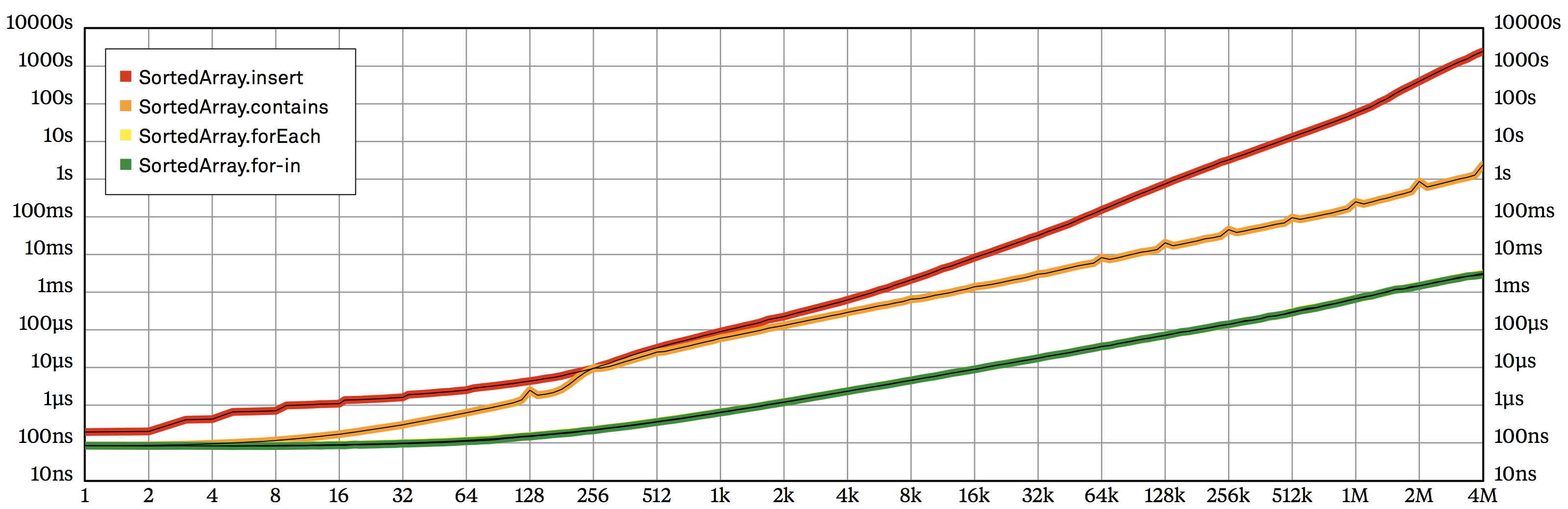
Such log-log plots are usually the best way to display benchmarking results. They fit a huge range of data on a single chart without letting large values overwhelm small ones — in this case, we can easily compare execution times from a single element, up to 4 million of them: a difference of 22 binary orders of magnitude!

Additionally, log-log plots make it easy to estimate the actual complexity costs an algorithm exhibits. If a section of a benchmark plot is a straight line segment, then the relationship between input size and execution time can be approximated by a multiple of a simple polynomial function, such as \(n\), \(n^2\), or even \(\sqrt n\). The exponent is related to the slope of the line: the slope of \(n^2\) is double that of \(n\). With some practice, you’ll be able to recognize the most frequently occurring relationships at a glance — there’s no need for complicated analysis.

In our case, we know that simply iterating over all the elements inside an array should take \(O(n)\) time, and this is confirmed by the plots. Array.forEach and the for-in loop cost pretty much the same, and after an initial warmup period, they both become straight lines. It takes a little more than three steps to the right for the line to go a single step up, which corresponds to \(2^{3.3} \approx 10\), proving a simple linear relationship.

Looking at the plot for SortedArray.insert, we find it gradually turns into a straight line at about 4,000 elements, and the slope of the line is roughly double that of SortedArray.forEach — so it looks like the execution time of insertion is a quadratic function of the input size. Luckily, this matches our expectations: each time we insert a random element into a sorted array, we have to make space for it by moving (on average) half of the existing elements one slot to the right. So a single insertion is a linear operation, which makes \(n\) insertions cost \(O(n^2)\).

SortedArray.contains does \(n\) binary searches, each taking \(O(\log n)\) time, so it’s supposed to be an \(O(n\log n)\) function. It’s hard to see this in figure 2.1, but you can verify it if you look close enough: its curve is almost parallel to that of forEach, except it subtly drifts upward — it’s not a perfectly straight line. One easy way to verify this is by putting the edge of a piece of paper next to the contains plot: it curves away from the paper’s straight edge, indicating a superlinear relationship.

To highlight the difference between \(O(n)\) and \(O(n\log n)\) functions, it’s useful to divide execution times by the input size, resulting in a chart that displays the average execution time spent on a single element. (I like to call this type of plot an amortized chart. I’m not sure the word amortized fits this context, but it does sound impressive!) The division eliminates the consistent slope of \(O(n)\), making it easier to distinguish linear and logarithmic factors. Figure 2.2 shows such a chart for SortedArray. 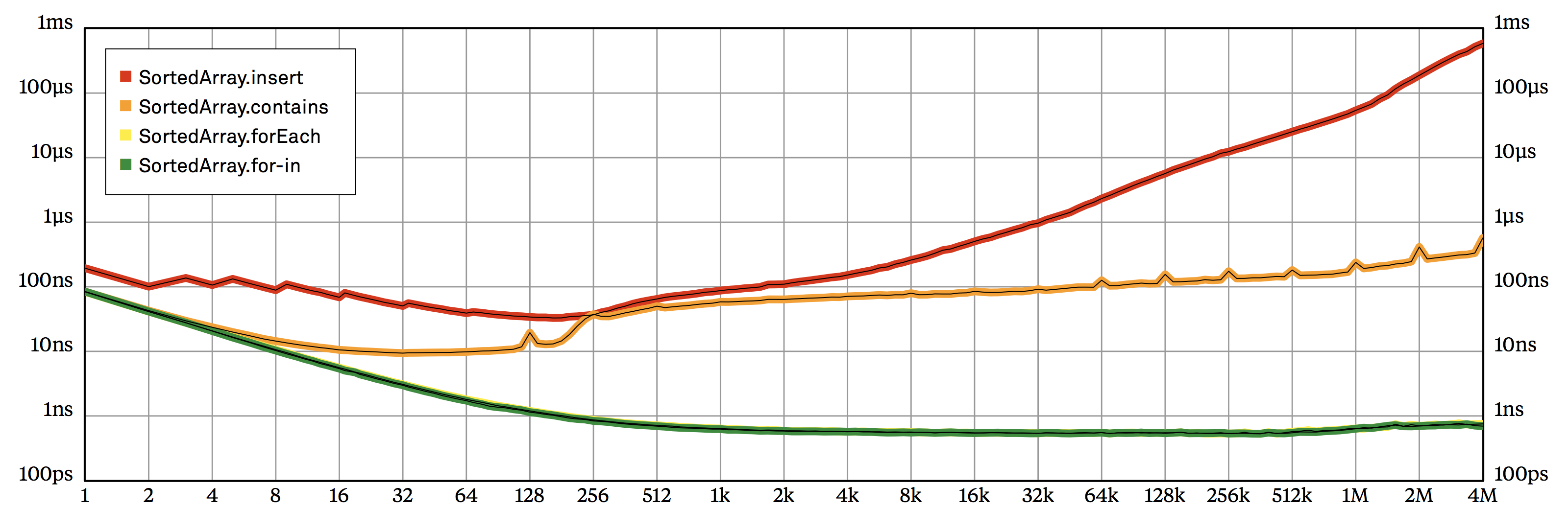Note how contains now has a distinct (if slight) upward slope, while the tail of forEach is perfectly flat.

The curve for contains has a couple of surprises. First, it has clear spikes at powers-of-two sizes. This is due to an interesting interaction between binary search and the architecture of the level 2 (L2) cache in the MacBook running the benchmarks. The cache is divided into 64-byte lines, each of which may hold the contents of main memory from a specific set of physical addresses. By an unfortunate coincidence, if the storage size is close to a perfect power of two, successive lookup operations of the binary search algorithm tend to all fall into the same L2 cache line, quickly exhausting its capacity, while other lines remain unused. This effect is called cache line aliasing, and it can evidently lead to a quite dramatic slowdown: contains takes about twice as long to execute at the top of the spikes than at nearby sizes.

One way to eliminate these spikes is to switch to ternary search, dividing the buffer into three equal slices on each iteration. An even simpler solution is to perturb binary search, selecting a slightly off-center middle index. To do this, we just need to modify a single line in the implementation of index(for:), adding a small extra offset to the middle index:

This way, the middle index will fall \(33/64\) the way between the two endpoints, which is enough to prevent cache line aliasing. Unfortunately, the code is now a tiny bit more complicated, and these off-center middle indices generally result in slightly more storage lookups than regular binary search. So the price of eliminating the power-of-two spikes is a small overall slowdown, as demonstrated: by the chart in figure 2.3.

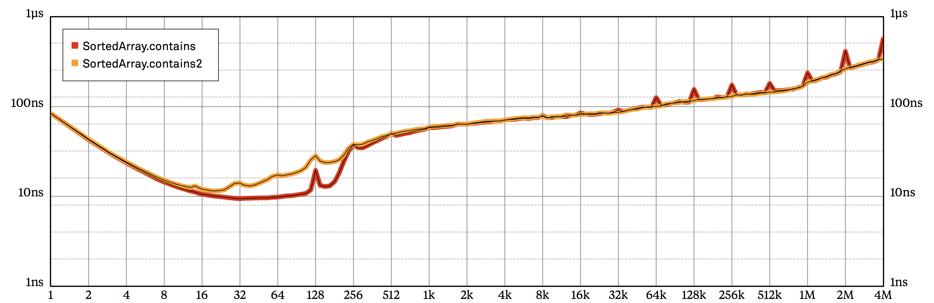
The other surprise of the contains curve is that it seems to turn slightly upward at about 64k elements or so. (If you look closely, you may actually detect a similar, although less pronounced, slowdown for insert, starting at about a million elements.) At this size, my MacBook’s virtual memory subsystem was unable to keep the physical address of all pages of the storage array in the CPU’s address cache (called the Translation Lookaside Buffer, or TLB for short). The contains benchmark randomizes lookups, so its irregular access patterns lead to frequent TLB cache misses, considerably increasing the cost of memory accesses. Additionally, as the storage array gets larger, its sheer size overwhelms L1 and L2 caches, and those cache misses contribute a great deal of additional latency.

At the end of the day, it looks like random memory accesses in a large enough contiguous buffer take \(O(\log n)\)-ish time, not \(O(1)\) — so the asymptotic execution time of our binary search is in fact more like \(O(\log n\log n)\), and not \(O(\log n)\) as we usually believe. Isn’t that interesting? (The slowdown disappears if we remove the shuffling of the lookups array in the benchmark code above. Try it!)

On the other hand, for small sizes, the contains curve keeps remarkably close to insert. Some of this is just a side effect of the logarithmic scale: at their closest point, contains is still 80% faster than insertion. But the insert curve looks surprisingly flat up to about 1,000 elements; it seems that as long as the sorted array is small enough, the average time it takes to insert a new element into it is basically independent of the size of the array. (I believe this is mostly a consequence of the fact that at these sizes, the entire array fits into the L1 cache of the CPU.)

So SortedArray.insert seems to be astonishingly fast as long as the array is small. For now, we can file this factoid away as mildly interesting trivia. Keep it in mind though, because this fact will have serious consequences in later parts of this book.

3 The Swiftification of NSOrderedSet

The Foundation framework includes a class called NSOrderedSet. It’s a relatively recent addition, first appearing in 2011 with iOS 5 and OS X 10.7 Lion. NSOrderedSet was added to Foundation specifically in support of ordered relationships in Core Data. It works like a combination of NSArray and NSSet, implementing the API of both classes. It also provides both NSSet’s super fast \(O(1)\) membership checks and NSArray’s speedy \(O(1)\) random access indexing. The tradeoff is that it also inherits NSArray’s \(O(n)\) insertions. Because NSOrderedSet is (most likely) implemented by wrapping an NSSet and an NSArray, it also has a higher memory overhead than either of these components.

NSOrderedSet hasn’t been bridged to Swift yet, so it seems like a nice subject for demonstrating how we can define thin wrappers around existing Objective-C classes to bring them closer to the Swift world.

Despite its promising name, NSOrderedSet isn’t really a good match for our use case. Although NSOrderedSet does keep its elements ordered, it doesn’t enforce any particular ordering relation — you can insert elements in whichever order you like and NSOrderedSet will remember it for you, just like an array. Not having a predefined ordering is the difference between “ordered” and “sorted,” and this is why NSOrderedSet is not called NSSortedSet. Its primary purpose is to make lookup operations fast, but it achieves this using hashing rather than comparisons. (There’s no equivalent to the Comparable protocol in Foundation; NSObject only provides the functionality of Equatable and Hashable.)

But if NSOrderedSet supports whichever ordering we may choose to use, then it also supports keeping elements sorted according to their Comparable implementation. Clearly, this won’t be the ideal use case for NSOrderedSet, but we should be able to make it work. So let’s import Foundation and start working on hammering NSOrderedSet into a SortedSet:

Right off the bat, we run into a couple of major problems.

First, NSOrderedSet is a class, so its instances are reference types. We want our sorted sets to have value semantics.

Second, NSOrderedSet is a heterogeneous sequence — it takes Any members. We could still implement SortedSet by setting its Element type to Any, rather than leaving it as a generic type parameter, but that wouldn’t feel like a real solution. What we really want is a generic homogeneous collection type, with the element type provided by a type parameter.

So we can’t just extend NSOrderedSet to implement our protocol. Instead, we’re going to define a generic wrapper struct that internally uses an NSOrderedSet instance as storage. This approach is similar to what the Swift standard library does in order to bridge NSArray, NSSet, and NSDictionary instances to Swift’s Array, Set, and Dictionary values. So we seem to be heading down the right track.

What should we call our struct? It’s tempting to call it NSSortedSet, and it would technically be possible to do so — Swift-only constructs don’t depend on prefixes to work around (present or future) naming conflicts. On the other hand, for developers, NS still implies Apple-provided, so it’d be impolite and confusing to use it. Let’s just go the other way and name our struct OrderedSet. (This name isn’t quite right either, but at least it does resemble the name of the underlying data structure.)

We want to be able to mutate our storage, so we need to declare it as an instance of NSMutableOrderedSet, which is NSOrderedSet’s mutable subclass.

3.1 Looking Up Elements

We now have the empty shell of our data structure. Let’s begin to fill it with content, starting with the two lookup methods, forEach and contains.

NSOrderedSet implements Sequence, so it already has a forEach method. Assuming elements are kept in the correct order, we can simply forward forEach calls to storage. However, we need to manually downcast values provided by NSOrderedSet to the correct type:

OrderedSet is in full control of its own storage, so it can guarantee the storage will never contain anything other than an Element. This ensures the forced downcast will always succeed. But it sure is ugly!

NSOrderedSet also happens to provide an implementation for contains, and it seems perfect for our use case. In fact, it’s simpler to use than forEach because there’s no need for explicit casting:

The code above compiles with no warnings, and it appears to work great when Element is Int or String. However, as we already mentioned, NSOrderedSet uses NSObject’s hashing API to speed up element lookups. But we don’t require Element to be Hashable! How could this work at all?

When we supply a Swift value type to a method taking an Objective-C object — as with storage.contains above, the compiler needs to box the value in a private NSObject subclass that it generates for this purpose. Remember that NSObject has built-in hashing APIs; you can’t have an NSObject instance that doesn’t support hash. So these autogenerated bridging classes must always have an implementation for hash that’s consistent with isEqual(:).

If Element happens to be Hashable, then Swift is able to use the type’s own == and hashValue implementations in the bridging class, so Element values get hashed the same way in Objective-C as in Swift, and everything works out perfectly.

However, if Element doesn’t implement hashValue, then the bridging class has no choice but to use the default NSObject implementations of both hash and isEqual(_:). Because there’s no other information available, these are based on the identity (i.e. the physical address) of the instances, which is effectively random for boxed value types. So two different bridged instances holding the exact same value will never be considered isEqual(_:) (or return the same hash).

The upshot of all this is that the above code for contains compiles just fine, but it has a fatal bug: if Element isn’t Hashable, then it always returns false. Oops!

Oh dear. Lesson of the day: be very, very careful when using Objective-C APIs from Swift. Automatic bridging of Swift values to NSObject instances is extremely convenient, but it has subtle pitfalls. There’s nothing in the code that explicitly warns about this problem: no exclamation marks, no explicit cast, nothing.

Well, now we know we can’t rely on NSOrderedSet’s own lookup methods in our case. Instead we have to look for some alternative APIs to find elements. Thankfully, NSOrderedSet also includes a method that was specifically designed for looking up elements when we know they’re sorted according to some comparator function:

Presumably this implements some form of binary search, so it should be fast enough. Our elements are sorted according to their Comparable implementation, so we can use Swift’s < and > operators to define a suitable comparator function:

We can use this comparator to define a method for getting the index for a particular element. This happens to be what Collection’s index(of:) method is supposed to do, so let’s make sure our definition refines the default implementation of it:

Once we have this function, contains reduces to a tiny transformation of its result:

I don’t know about you, but I found this a lot more complicated than I originally expected. The fine details of how values are bridged into Objective-C sometimes have far-reaching consequences that may break our code in subtle but fatal ways. If we aren’t aware of these wrinkles, we may be unpleasantly surprised.

NSOrderedSet’s flagship feature is that its contains implementation is super fast — so it’s rather sad that we can’t use it. But there’s still hope! Consider that while NSOrderedSet.contains may mistakenly report false for certain types, it never returns true if the value isn’t in fact in the set. Therefore, we can write a variant of OrderedSet.contains that still calls it as a shortcut, possibly eliminating the need for binary search:

For Hashable elements, this variant will return true faster than index(of:). However, it’s slightly slower for values that aren’t members of the set and for types that aren’t hashable.

3.2 Implementing Collection

NSOrderedSet only conforms to Sequence, and not to Collection. (This isn’t some unique quirk; its better-known friends NSArray and NSSet do the same.) Nevertheless, NSOrderedSet does provide some integer-based indexing methods we can use to implement RandomAccessCollection in our OrderedSet type:

This turned out to be refreshingly simple.

4 Red-Black Trees

Self-balancing binary search trees provide efficient algorithms for implementing sorted collections. In particular, these data structures can be used to implement sorted sets so that the insertion of any element only takes logarithmic time. This is a really attractive feature — remember, our SortedArray implemented insertions in linear time.

The expression, “self-balancing binary search tree,” looks kind of technical. Each word has a specific meaning, so I’ll quickly explain them.

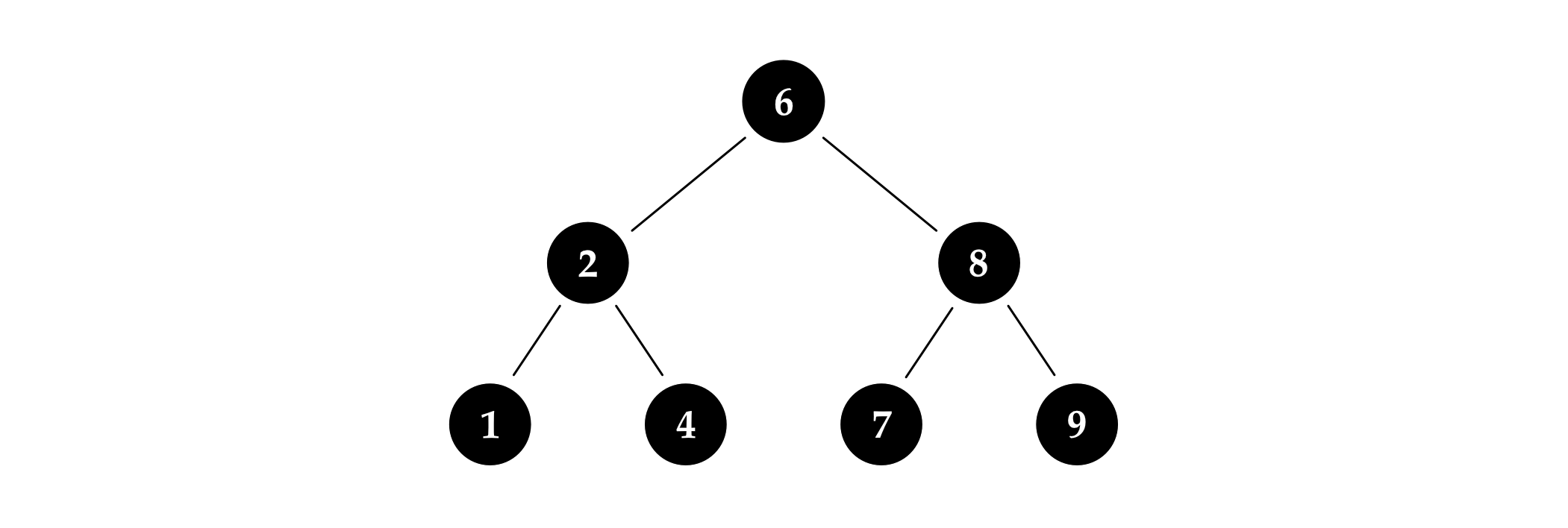
A tree is a data structure with data stored inside nodes, arranged in a branching, tree-like structure. Each tree has a single node at the top called the root node. (The root is put on the top because computer scientists have been drawing trees upside down for decades. This is because it’s more practical to draw tree diagrams this way, and not because they don’t know what an actual tree looks like. Or at least I hope so, anyway.) If a node has no children, then it’s called a leaf node; otherwise, it’s an internal node. A tree usually has many leaf nodes.

In general, internal nodes may have any number of child nodes, but in binary trees, nodes may only have two children, called left and right. Some nodes may have two children, while some may have only a left child, only a right child, or no child at all.

In search trees, the values inside nodes are comparable in some way, and nodes are arranged such that for every node in the tree, all values inside the left subtree are less than the value of the node, and all values to the right are greater than it. This makes it easy to find any particular element.

By self-balancing, we mean that the data structure has some sort of mechanism that guarantees the tree remains nice and bushy with a short height, no matter which values it contains and in what order the values are inserted. If the tree was allowed to grow lopsided, even simple operations could become inefficient. (As an extreme example, a tree where each node has at most one child works like a linked list — not very efficient at all.)

There are many ways to create self-balancing binary trees; in this section, we’re going to implement the variant called red-black trees. This particular flavor needs to store a single extra bit of information in every node to implement the self-balancing part. That extra bit is the node’s color, which can be either red or black.

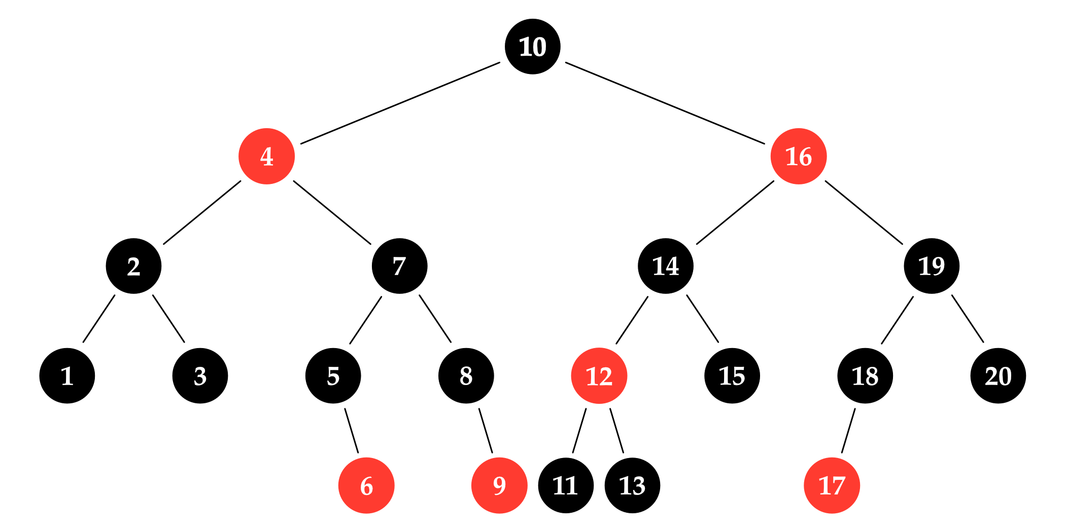
A red-black tree always keeps its nodes arranged and colored so that the following properties are all true:

1. The root node is black.
2. Red nodes only have black children. (If they have any, that is.)
3. Every path from the root node to an empty spot in the tree contains the same number of black nodes.

Empty spots are places where new nodes can be added to the tree, i.e. where a node has no left or right child. To grow a tree one node larger, we just need to replace one of its empty spots with a new node.

The first property is there to make our algorithms a little bit simpler; it doesn’t really affect the tree’s shape at all. The last two properties ensure that the tree remains nicely dense, where no empty spot in the tree is more than twice as far from the root node as any other.

To fully understand these balancing properties, it’s useful to play with them a little, exploring their edge cases. For example, it’s possible to construct a red-black tree that consists solely of black nodes; the tree in figure 4.3 is one example.

If we try to construct more examples, we’ll soon realize that the third red-black property restricts such trees into a particular shape where all internal nodes have two children and all leaf nodes are on the same level. Trees with this shape are called perfect trees because they’re so perfectly balanced and symmetrical. This is the ideal shape all balanced trees aspire to, because it puts every node as close to the root as possible.

Unfortunately, it’d be unreasonable to require balancing algorithms to maintain perfect trees: indeed, it’s only possible to construct perfect binary trees with certain node counts. There’s no perfect binary tree with four nodes, for example.

To make red-black trees practical, the third red-black property therefore uses a weaker definition of balancing, where red nodes aren’t counted. However, to make sure things don’t get too unruly, the second property limits the number of red nodes to something reasonable: it ensures that on any particular path in the tree, the number of red nodes will never exceed the number of black ones.

5 The Copy-On-Write Optimization

RedBlackTree creates a brand-new tree every time we insert a new element. The new tree shares some of its nodes with the original, but nodes on the entire path from the root to the new node are replaced with newly allocated nodes. This is the “easy” way to implement value semantics, but it’s a bit wasteful.

When the nodes of a tree value aren’t shared between other values, it’s OK to mutate them directly — nobody will mind, because nobody else knows about that particular tree instance. Direct mutation will eliminate most of the copying and allocation, often resulting in a dramatic speedup.

We’ve already seen how Swift supports implementing optimized copy-on-write value semantics for reference types by providing the isKnownUniquelyReferenced function. Unfortunately, Swift 4 doesn’t give us tools to implement COW for algebraic data types. We don’t have access to the private reference type Swift uses to box up nodes, so we have no way to determine if a particular node is uniquely referenced. (The compiler itself doesn’t have the smarts (yet?) to do the COW optimization on its own either.) There’s also no easy way to directly access a value stored inside an enum case without extracting a separate copy of it. (Note that Optional does provide direct access to the value stored in it via its forced unwrapping ! operator. However, the tools for implementing similar in-place access for our own enum types aren’t available for use outside the standard library.)

So to implement COW, we need to give up on our beloved algebraic data types for now and rewrite everything into a more conventional (dare I say tedious?) imperative style, using boring old structs and classes, with a sprinkle of optionals.

5.1 Basic Definitions

First, we need to define a public struct that’ll represent sorted set values. The RedBlackTree2 type below is just a small wrapper around a reference to a tree node that serves as its storage. OrderedSet worked the same way, so this pattern is already quite familiar to us by now:

Next, let’s take a look at the definition of our tree nodes:

Beyond the fields we had in the original enum case for RedBlackTree.node, this class also includes a new property called mutationCount. Its value is a count of how many times the node was mutated since its creation. This will be useful in our Collection implementation, where we’ll use it to create a new design for indices. (We explicitly use a 64-bit integer so that it’s unlikely the counter will ever overflow, even on 32-bit systems. Storing an 8-byte counter in every node isn’t really necessary, as we’ll only use the value stored inside root nodes. Let’s ignore this fact for now; it’s simpler to do it this way, and we’ll find a way to make this less wasteful in the next chapter.)

But let’s not jump ahead!

Using a separate type to represent nodes vs. trees means we can make the node type a private implementation detail to the public RedBlackTree2. External users of our collection won’t be able to mess around with it, which is a nice bonus — everybody was able to see the internals of RedBlackTree, and anyone could use Swift’s enum literal syntax to create any tree they wanted, which would easily break our red-black tree invariants.

The Node class is an implementation detail of the RedBlackTree2 struct; nesting the former in the latter expresses this relationship neatly. This also prevents naming conflicts with other types named Node in the same module. Additionally, it simplifies the syntax a little bit: Node automatically inherits RedBlackTree2’s Element type parameter, so we don’t have to explicitly specify it.

Again, tradition dictates that the 1-bit color property should be packed into an unused bit in the binary representation of one of Node’s reference properties; but it’d be unsafe, fragile, and fiddly to do that in Swift. It’s better to simply keep color as a standalone stored property and to let the compiler set up storage for it.

Note that we essentially transformed the two-case RedBlackTree enum into optional references to the Node type. The .empty case is represented by a nil optional, while a non-nil value represents a .node. Node is a heap-allocated reference type, so we’ve made the previous solution’s implicit boxing an explicit feature, giving us direct access to the heap reference and enabling the use of isKnownUniquelyReferenced.

6 B-Trees

The raw performance of a small sorted array seems impossible to beat. So let’s not even try; instead, let’s build a sorted set entirely out of small sorted arrays!

It’s easy enough to get started: we just insert elements into a single array until we reach some predefined maximum size. Let’s say we want to keep our arrays below five elements and we’ve already inserted four values:

 

If we now need to insert the value 10, we get an array that’s too large:

 

We can’t keep it like this, so we have to do something. One option is to cut the array into two halves, extracting the middle element to serve as a sort of separator value between them:

 

Now we have a cute little tree structure with leaf nodes containing small sorted arrays. This seems like a promising approach: it combines sorted arrays and search trees into a single unified data structure, hopefully giving us array-like super-fast insertions at small sizes, all while retaining tree-like logarithmic performance for large sets. Synergy!

Let’s see what happens when we try adding more elements. We can keep inserting new values in the two leaf arrays until one of them gets too large again:

 

When this happens, we need to do another split, giving us three arrays and two separators:

 

What should we do with those two separator values? We store all other elements in sorted arrays, so it seems like a reasonable idea to put these separators in a sorted array of their own:

 

So apparently each node in our new array-tree hybrid will hold a small sorted array. Nice and consistent; I love it so far.

Now let’s say we want to insert the value 20 next. This goes in the rightmost array, which already has four elements — so we need to do another split, extracting 16 from the middle as a new separator. No biggie, we can just insert it into the array at the top:

 

Lovely! We can keep going like this; inserting 25, 26, and 27 overflows the rightmost array again, extracting the new separator, 25:

 

However, the top array is now full, which is worrying. Let’s say we insert 18, 21, and 22 next, so we end up with the situation below:

 

What next? We can’t leave the separator array bloated like this. Previously, we handled oversized arrays by splitting them — why not try doing the same now?

 

Oh, how neat: splitting the second-level array just adds a third level to our tree. This gives us a way to keep inserting new elements indefinitely; when the third-level array fills up, we can just add a fourth level, and so on, ad infinitum:

 

We’ve just invented a brand-new data structure! This is so exciting.

Unfortunately, it turns out that Rudolf Bayer and Ed McCreight already had the same idea way back in 1971, and they named their invention B-tree. What a bummer! I wrote an entire book to introduce a thing that’s almost half a century old. How embarrassing.

Fun fact: red-black trees were actually derived from a special case of B-trees in 1978. These are all ancient data structures.

6.1 B-Tree Properties

As we’ve seen, B-trees are search trees like red-black trees, but their layout is different. In a B-tree, nodes may have hundreds (or even thousands) of children, not just two. The number of children isn’t entirely unrestricted, though: this number must fit inside a certain range.

The maximum number of children a node may have is determined when the tree is created — this number is called the order of a B-tree. (The order of a B-tree has nothing to do with the ordering of its elements.) Note that the maximum number of elements stored in a node is one less than the tree’s order. This can be a source of off-by-one indexing errors, so it’s important to keep in mind as we work on B-tree internals.

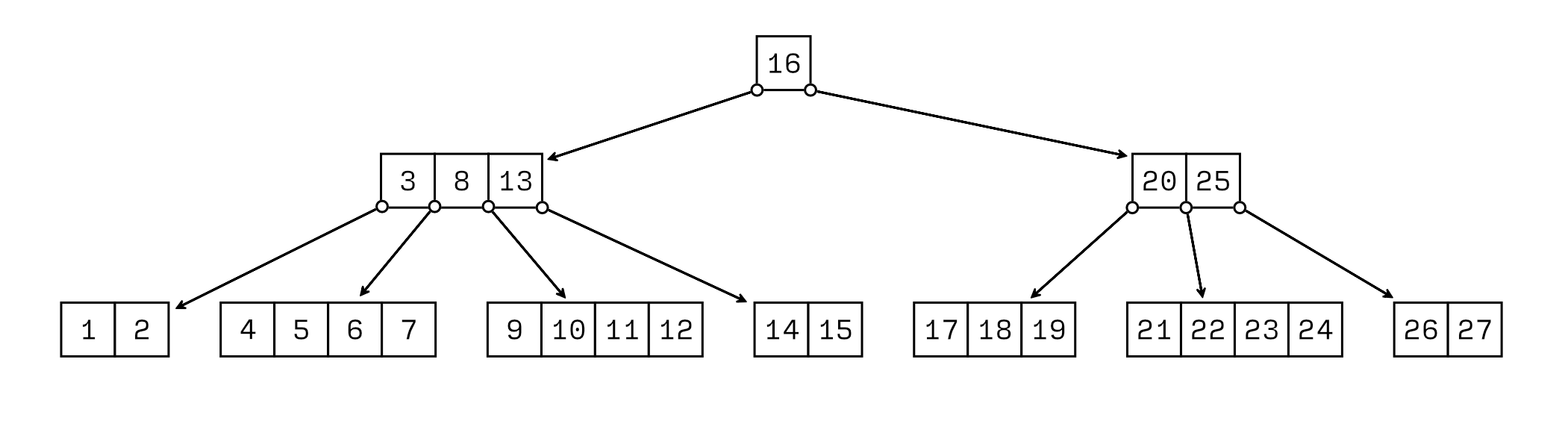
In the previous section, we built an example B-tree of order 5. In practice, the order is typically between 100 and 2,000, so 5 is unusually low. However, nodes with 1,000 children wouldn’t easily fit on the page; it’s easier to understand B-trees by drawing toy examples.

To help in finding our way inside the tree, each internal node stores one element between each of its children, similar to how a node in a red-black tree contains a single value sorted between its left and right subtrees. So a B-tree node with 1,000 children will contain 999 elements neatly sorted in increasing order.

To keep lookup operations fast, B-trees maintain the following balancing invariants:

1. Maximum size: All nodes store a maximum of order - 1 elements, sorted in increasing order.

2. Minimum size: Non-root nodes must never be less than half full, i.e. the number of elements in all nodes except the root node must be at least (order - 1) / 2.

3. Uniform depth: All leaf nodes must be at the same depth in the tree, counting from the root node at the top.

Note that the last two properties are a natural consequence of the way we do insertions; we didn’t have to do anything special to prevent nodes from getting too small or to make sure all leaves are on the same level. (These properties are much harder to maintain in other B-tree operations, though. For instance, removing an element may result in an undersized node that needs to be fixed.)

According to these rules, nodes in a B-tree of order 1,000 will hold anywhere between 499 and 999 elements (inclusive). The single exception is the root node, which isn’t constrained by the lower bound: it may contain 0 to 999 elements. (This is so we can create B-trees with, say, less than 499 elements.) Therefore, a single B-tree node on its own may have the same number of elements as a red-black tree that is 10–20 levels deep!

Storing so many elements in a single node has two major advantages:

1. Reduced memory overhead. Each value in a red-black tree is stored in a separate, heap-allocated node that also includes a pointer to a method lookup table, its reference count, and the two references for the node’s left and right children. Nodes in a B-tree store elements in bulk, which can considerably reduce memory allocation overhead. (The exact savings depends on the size of the elements and the order of the tree.)

2. Access patterns better suited for memory caching. B-tree nodes store their elements in small contiguous buffers. If the buffers are sized so that they fit well within the L1 cache of the CPU, operations working on them can be considerably faster than the equivalent code operating on red-black trees, the values of which are scattered all over the heap.

To understand how dense B-trees really are, consider that adding an extra level to a B-tree multiplies the maximum number of elements it may store by its order. For example, here’s how the minimum and maximum element counts grow as we increase the depth of a B-tree of order 1,000:

Depth	Minimum size	Maximum size
1	0	999
2	999	999 999
3	499 999	999 999 999
4	249 999 999	999 999 999 999
5	124 999 999 999	999 999 999 999 999
6	62 499 999 999 999	999 999 999 999 999 999
⋮	⋮	⋮
\(n\)	\(2 {\left\lceil\frac{order}{2}\right\rceil}^{n-1}-1\)	\(order^{n} - 1\)

Clearly, we’ll rarely, if ever, work with B-trees that are more than a handful of levels deep. Theoretically, the depth of a B-tree is \(O(\log n)\), where \(n\) is the number of elements. But the base of this logarithm is so large that, given the limited amount of memory available in any real-world computer, it’s in fact not too much of a stretch to say that B-trees have \(O(1)\) depth for any input size we may reasonably expect to see in practice.

This last sentence somehow seems to make sense, even though the same line of thinking would lead me to say that any practical algorithm runs in \(O(1)\) time, with the constant limit being my remaining lifetime — obviously, I don’t find algorithms that finish after my death very practical at all. On the other hand, you could arrange all particles in the observable universe into a 1,000-order B-tree that’s just 30 levels or so deep; so it does seem rather pointless and nitpicky to keep track of the logarithm.

Another interesting consequence of such a large fan-out is that in B-trees, the vast majority of elements are stored in leaf nodes. Indeed, in a B-tree of order 1,000, at least 99.8% of elements will always reside in leaves. Therefore, for operations that process B-tree elements in bulk (such as iteration), we mostly need to concentrate our optimization efforts on making sure leaf nodes are processed fast: the time spent on internal nodes often won’t even register in benchmarking results.

Weirdly, despite this, the number of nodes in a B-tree is still technically proportional to the number of its elements, and most B-tree algorithms have the same “big-O” performance as the corresponding binary tree code. In a way, B-trees play tricks with the simplifying assumptions behind the big-O notation: constant factors often do matter in practice. This should be no surprise by now. After all, if we didn’t care about constant factors, we could’ve ended this book after the chapter on RedBlackTree!

7 Additional Optimizations

In this chapter, we’re going to concentrate on optimizing BTree.insert even further, squeezing our code to get the last few drops of sweet performance out.

We’ll create three more SortedSet implementations, creatively naming them BTree2, BTree3, and BTree4. To keep this book at a manageable length, we aren’t going to include the full source code of these three B-tree variants; we’ll just describe the changes through a few representative code snippets. You can find the full source code for all three B-tree variants in the book’s GitHub repository.

If you’re bored with SortedSets, it’s OK to skip this chapter, as the advanced techniques it describes are rarely applicable to everyday app development work.

7.1 Inlining Array’s Methods

BTree stores elements and children of a Node in standard Arrays. In the last chapter, this made the code relatively easy to understand, which helped us explain B-trees. However, Array includes logic for index validation and COW that is redundant inside BTree — supposing we didn’t make any coding mistakes, BTree never subscripts an array with an out-of-range index, and it implements its own COW behavior.

Looking at our insertion benchmark chart (figure 7.1), we see that while BTree.insert is extremely close to SortedArray.insert at small set sizes, there’s still a 10–20% performance gap between them. Would eliminating Array’s (tiny) overhead be enough to close this gap? Let’s find out!

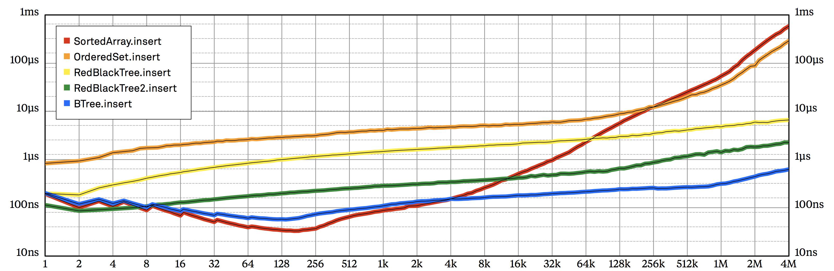
The Swift standard library includes UnsafeMutablePointer and UnsafeMutableBufferPointer types we can use to implement our own storage buffers. They deserve their scary names; working with these types is only slightly easier than working with C pointers — the slightest mistake in the code that handles them may result in hard-to-debug memory corruption bugs, memory leaks, or even worse! On the other hand, if we promise to be super careful, we might be able to use these to slightly improve performance.

8 Conclusion

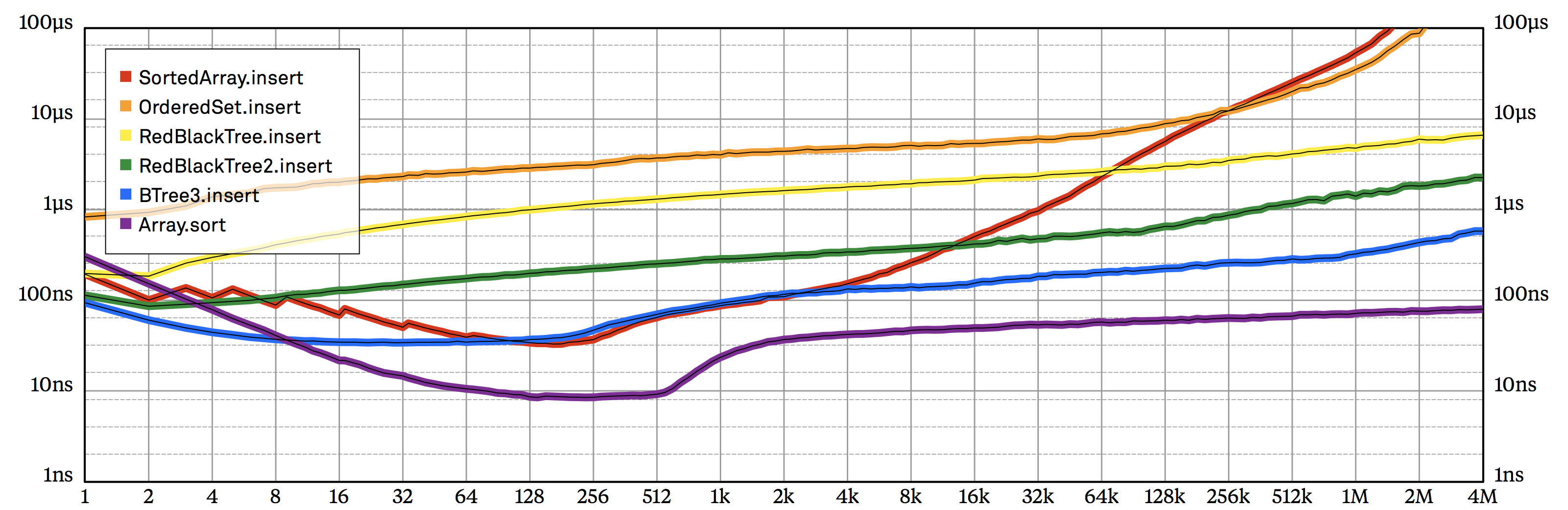
In this book, we’ve discussed seven different ways to implement the same simple collection type. Every time we created a new solution, our code became incrementally more complicated, but in exchange, we gained substantial performance improvements. This is perhaps best demonstrated by the steady downward progress of our successive insertion implementations on the benchmark chart.

Is it possible to implement an even faster SortedSet.insert? Well, BTree3 certainly has room for some additional micro-optimizations; I think a 5–10% improvement is definitely possible. Investing even more effort would perhaps get us 20%.

But is it possible we missed some clever optimization trick that would get us another huge performance jump of 200–400%? I don’t believe so.

First of all, note that by inserting a bunch of elements into a sorted set, we’re essentially sorting them. We could also do that by simply calling Array.sort, which implements the super speedy Introsort sorting algorithm. The last line in the chart above depicts the amortized time Array.sort spends on each element. In a very real sense, Array.sort sets a hard upper limit on the performance we can expect out of any sorted set.

At typical sizes, sorting elements by calling BTree3.insert in a loop is just 3.5 times slower than Array.sort. This is already amazingly close! Consider that the BTree3 benchmark processes each element individually and keeps existing elements neatly sorted after each insertion. I find it surprising that BTree3.insert gets so close despite such a huge handicap, and I’d be shocked to learn about a new SortedSet implementation that improves on B-trees by even 50%.

8.1 Implementing Insertion in Constant Time

Although it may not be possible to drastically improve on BTree3 while fully implementing all SortedSet requirements, we can always speed things up by cheating!

For example, SillySet in the code below implements the syntactic requirements of the SortedSet protocol with an insert method that takes \(O(1)\) time. It runs circles around Array.sort in the insert benchmark above without even breaking a sweat:

Of course, there are many problems with this code: for example, it requires Element to be hashable, and it violates Collection requirements by implementing subscript in \(O(n \log n)\) time — which is absurdly long. But the problem I find most vexing is that SillySet’s indexing subscript modifies its underlying storage by side effect — this breaks my assumptions about what value semantics mean in Swift. (For example, it makes it dangerous to pass SillySet values between threads; even read-only concurrent access may result in data races.)

This particular example might be silly, but the idea of deferring the execution of successive insertions by collecting such elements into a separate buffer has a lot of merit. Creating a sorted set by individually inserting a bunch of elements in a loop isn’t very efficient at all. It’s a lot quicker to first sort the elements in a separate buffer and then use special bulk loading initializers to convert the buffer into a B-tree in linear time.

Bulk loading works by exploiting the fact that we don’t care whether its intermediate states satisfy sorted set requirements — we never look at elements of a half-loaded set.

It’s important to recognize opportunities for this type of optimization, because they allow us to temporarily escape our usual constraints, often resulting in performance boosts that wouldn’t otherwise be possible.

8.2 Farewell

I hope you enjoyed reading this book! I had a lot of fun putting it together. Along the way, I learned a great deal about implementing collections in Swift, and hopefully you picked up a couple of new tricks too.

Throughout this book, we explored a number of different ways to solve the particular problem of building a sorted set, concentrating on benchmarking our solutions in order to find ways to improve their performance.

However, none of our implementations were complete, as the code we wrote was never really good enough for production use. To keep the book relatively short and to the point, we took some shortcuts that would be inappropriate to take in a real package.

Indeed, even our SortedSet protocol was simplified to the barest minimum: we cut most of the methods of SetAlgebra. For instance, we never discussed how to implement the remove operation. Somewhat surprisingly, it’s usually much harder to remove elements from a balanced tree than it is to insert them. (Try it!)

We didn’t spend time examining all the other data types we can build out of balanced search trees. Tree-based sorted maps, lists, and straightforward variants like multisets and multimaps are just as important as sorted sets; it would’ve been interesting to see how our code could be adapted to implement them.

We also didn’t explain how these implementations could be tested. This is a particularly painful omission, because the code we wrote was often tricky, and we sometimes used unsafe constructs, where the slightest mistake could result in scary memory corruption issues and days of frustrating debugging work.

Testing is hugely important; unit tests in particular provide a safety net against regressions and are pretty much a prerequisite to any kind of optimization work. Data structures lend themselves to unit testing especially well: their operations take easy-to-generate input and they produce well-defined, easily validatable output. Powerful packages like SwiftCheck provide easy-to-use tools for providing full test coverage.

That said, testing COW implementations can be a challenging task. If we aren’t careful enough about not making accidental strong references before calling isKnownUniquelyReferenced, our code will still produce correct results — it will just do it a lot slower than we expect. We don’t normally check for performance issues like this in unit tests, and we need to specially instrument our code to easily catch them.

On the other hand, if we simply forget to ensure we don’t mutate shared storage, our code will also affect variables holding unmutated copies. This kind of unexpected action at a distance can be extremely hard to track down, because our operation breaks values that aren’t explicitly part of its input or output. To ensure we catch this error, we need to write unit tests that specifically check for it — normal input/output checks won’t necessarily detect it, even if we otherwise have 100% test coverage.

We did briefly mention that by adding element counts to the nodes of a search tree, we can find the \(i\)th smallest or largest element in the tree in \(O(\log n)\) time. This trick can in fact be generalized: search trees can be augmented to speed up the calculation of any associative binary operation over arbitrary ranges of elements. Augmentation is something of a secret weapon in algorithmic problem solving: it enables us to easily produce efficient solutions to many complicated-looking problems. We didn’t have time to explain how to implement augmented trees or how we might solve problems using them.

Still, this seems like a good point to end the book. We’ve found what seems to be the best data structure for our problem, and we’re now ready to start working on building it up and polishing it into a complete, production-ready package. This is by no means a trivial task: we looked at the implementation of half a dozen or so operations, but we need to write, test, and document dozens more!

If you liked this book and you’d like to try your hand at optimizing production-quality collection code, take a look my BTree package on GitHub. At the time of writing, the most recent version of this package doesn’t even implement some of the optimizations in our original B-tree code, much less any of the advanced stuff in Chapter 7. There’s lots of room for improvement, and your contributions are always welcome.

How This Book Was Made

This book was generated by bookie, my tool for creating books about Swift. (Bookie is of course the informal name for a bookmaker, so the name is a perfect fit.)

Bookie is a command-line tool written in Swift that takes Markdown text files as input and produces nicely formatted Xcode Playground, GitHub-flavored Markdown, EPUB, HTML, LaTeX, and PDF files, along with a standalone Swift package containing all the source code. It knows how to generate playgrounds, Markdown, and source code directly; the other formats are generated by pandoc after converting the text into pandoc’s own Markdown dialect.

To verify code samples, bookie extracts all Swift code samples into a special Swift package (carefully annotated with #sourceLocation directives) and builds the package using the Swift Package Manager. The resulting command-line app is then run to print the return value of all lines of code that are to be evaluated. This output is then split, and each individual result is inserted into printed versions of the book after its corresponding line of code:

(In playgrounds, such output is generated dynamically, but the printout has to be explicitly included in the other formats.)

Syntax coloring is done using SourceKit, like in Xcode. SourceKit uses the official Swift grammar, so contextual keywords are always correctly highlighted:

Ebook and print versions of this book are typeset in Tiempos Text by the Klim Type Foundry. Code samples are set in Laurenz Brunner’s excellent Akkurat.

Bookie is not (yet?) free/open source software; you need to contact us directly if you’re interested in using it in your own projects.