Many developers enjoy building OS X or iOS applications because of how quickly one can create a viable application using the Cocoa frameworks. Even complex applications can be designed and built by small teams, in large part because of the capabilities provided by the tools and frameworks on these platforms. Swift playgrounds build on this tradition of rapid development, and they have the potential to change the way that we design and write OS X and iOS applications.
For those not familiar with the concept, Swift playgrounds are interactive documents where Swift code is compiled and run live as you type. Results of operations are presented in a step-by-step timeline as they execute, and variables can be logged and inspected at any point. Playgrounds can be created within an existing Xcode project or as standalone bundles that run by themselves.
While a lot of attention has been focused on Swift playgrounds for their utility in learning this new language, you only need to look at similar projects like IPython notebooks to see the broader range of potential applications for interactive coding environments. IPython notebooks are being used today for tasks ranging from scientific research to experimenting with machine vision. They're also being used to explore other language paradigms, such as functional programming with Haskell.
We'll explore the use of Swift playgrounds for documentation, testing, and rapid prototyping. All Swift playgrounds used for this article can be downloaded here.
Playgrounds for Documentation and Testing
Swift is a brand new language, and many people are using playgrounds to understand its syntax and conventions. In addition to the language, we were provided with a new standard library. The functions in this standard library at present aren't documented particularly well, so resources like the practicalswift.org list of standard library functions have sprung up.
However, it's one thing to read about what a function should do and another to see it in action. In particular, many of these functions perform interesting actions on the new Swift collection classes, and it would be informative to examine how they act on these collections.
Playgrounds provide a great opportunity to document functions and library interfaces by showing syntax and live execution against real data sets. For the case of the collection functions, we've created the CollectionOperations.playground, which contains a list of these functions, all run against sample data that can be changed live.
As a sample, we create our initial array using this:
let testArray = [0, 1, 2, 3, 4]
We then want to demonstrate the filter() function, so we write the following:
								let odds = testArray.filter{$0 % 2 == 1}
odds
The last line triggers the display of the array that results from this operation: [1, 3]. You get syntax, an example, and an illustration of how the function works, all in a live document.
This is effective for other Apple or third-party frameworks as well. For example, Scene Kit is an excellent framework that Apple provides for quickly building 3D scenes on Mac and iOS, and you might want to show someone how to get started with it. You could provide a sample application, but that requires a build and compile cycle to demonstrate.
In the SceneKitMac.playground, we've built a fully functional 3D scene with an animating torus. You will need to show the Assistant Editor (View | Assistant Editor | Show Assistant Editor) to display the 3D view, which will automatically render and animate. This requires no compile cycle, and someone could play around with this to change colors, geometry, lighting, or anything else about the scene, and see it be reflected live. It documents and presents an interactive example for how to use this framework.
In addition to documenting functions and their operations, you'll also note that we can verify that a function still operates as it should by looking at the results it provides, or even whether it is still parsed properly when we load the playground. It's not hard to envision adding assertions and creating real unit tests within a playground. Taken one step further, tests could be created for desired conditions, leading to a style of test-driven development as you type.
In fact, in the July 2014 issue of the PragPub magazine, Ron Jeffries has this to say in his article, "Swift from a TDD Perspective":
The Playground will almost certainly have an impact on how we TDD. I think we’ll go faster, by using Playground’s ability to show us quickly what we can do. But will we go better, with the same solid scaffolding of tests that we’re used to with TDD? Or will we take a hit in quality, either through defects or less refactoring?
While the question about code quality is for others to answer, let's take a look at how playgrounds can speed up development through rapid prototyping.
Prototyping Accelerate — Optimized Signal Processing
The Accelerate framework contains powerful functions for parallel processing of large data sets. These functions take advantage of the vector-processing instructions present in modern CPUs, such as the SSE instruction set in Intel chips, or the NEON ones on ARM. However, for their power, their interfaces can seem opaque and documentation on their use is a little sparse. As a result, not as many developers take advantage of the libraries under Accelerate's umbrella.
Swift presents opportunities to make it much easier to interact with Accelerate through function overloading and the creation of wrappers around the framework. Chris Liscio has been experimenting with this in his SMUGMath library, which acted as the inspiration for this prototype.
Let's say you had a series of data samples that made up a sine wave, and you wanted to determine the frequency and amplitude of that sine wave. How would you do this? One way to find these values is by means of a Fourier transform, which can extract frequency and amplitude information from one or many overlapping sine waves. Accelerate provides a version of this, called a Fast Fourier Transform (FFT), for which a great explanation (with an IPython notebook) can be found here.
To prototype this process, we'll be using the AccelerateFunctions.playground, so you can follow along using that. Make sure you expose the Assistant Editor (View | Assistant Editor | Show Assistant Editor) to see the graphs generated at each stage.
The first thing to do is to generate some sample waveforms for us to experiment with. An easy way to do that is by the use of Swift's map() operator:
								let sineArraySize = 64

let frequency1 = 4.0
let phase1 = 0.0
let amplitude1 = 2.0
let sineWave = (0..<sineArraySize).map {
    amplitude1 * sin(2.0 * M_PI / Double(sineArraySize) * Double($0) * frequency1 + phase1)
}
For later use in the FFT, our starting waveform array sizes need to be powers of two. Adjusting the sineArraySize to values like 32, 128, or 256 will vary the resolution of the graphs presented later, but it won't change the fundamental results of the calculations.
To plot our waveforms, we'll use the new XCPlayground framework (which needs to be imported first) and the following helper function:
								func plotArrayInPlayground<T>(arrayToPlot:Array<T>, title:String) {
    for currentValue in arrayToPlot {
        XCPCaptureValue(title, currentValue)
    }
}
When we do this:
plotArrayInPlayground(sineWave, "Sine wave 1")
We see a graph that looks like the following:
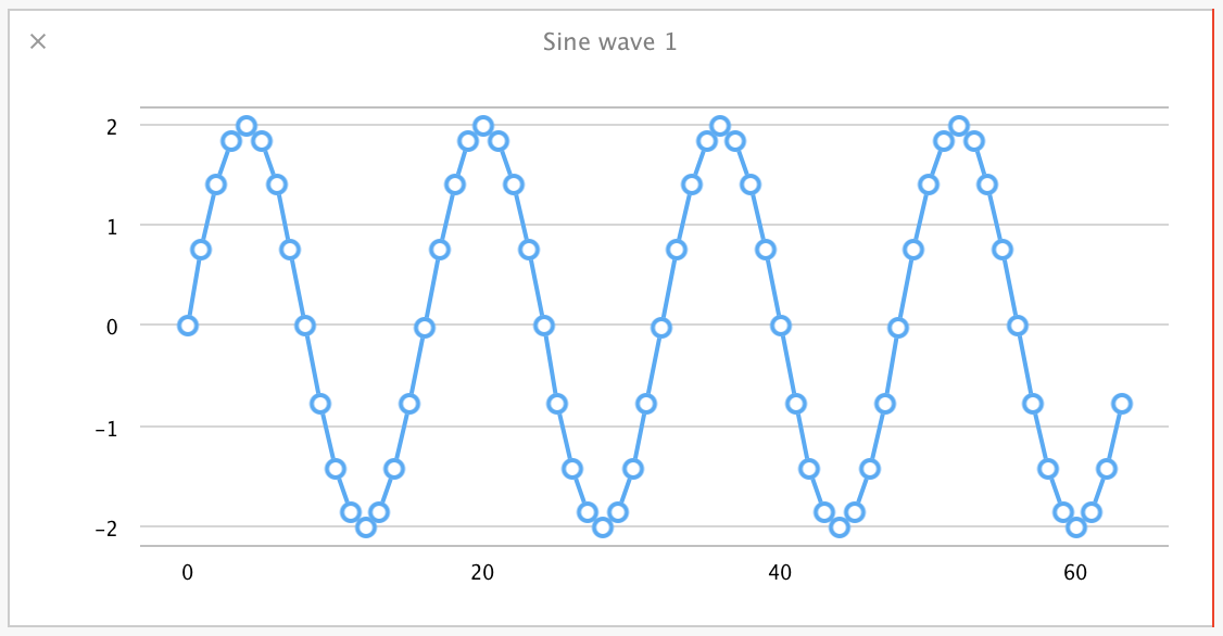
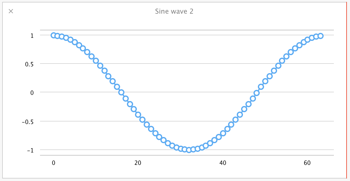
That's a sine wave with a frequency of 4.0, amplitude of 2.0, and phase of 0.0. Let's make this more interesting by creating a second sine wave to add to the first, this time of frequency 1.0, amplitude 1.0, and a phase of pi / 2.0:
								let frequency2 = 1.0
let phase2 = M_PI / 2.0
let amplitude2 = 1.0
let sineWave2 = (0..<sineArraySize).map {
    amplitude2 * sin(2.0 * M_PI / Double(sineArraySize) * Double($0) * frequency2 + phase2)
}
Now we want to combine them. This is where Accelerate starts to help us. Adding two arrays of independent floating-point values is well-suited to parallel processing. Accelerate's vDSP library has functions for just this sort of thing, so let's put them to use. For the fun of it, let's set up a Swift operator to use for this vector addition. Unfortunately, + is already used for array concatenation (perhaps confusingly so), and ++ is more appropriate as an increment operator, so we'll define a +++ operator for this vector addition:
								infix operator  +++ {}
func +++ (a: [Double], b: [Double]) -> [Double] {
    assert(a.count == b.count, "Expected arrays of the same length, instead got arrays of two different lengths")

    var result = [Double](count:a.count, repeatedValue:0.0)
    vDSP_vaddD(a, 1, b, 1, &result, 1, UInt(a.count))
    return result
}
This sets up an operator that takes in two Swift arrays of Double values and outputs a single combined array from their element-by-element addition. Within the function, a blank result array is created at the size of our inputs (asserted to be the same for both inputs). Because Swift arrays of scalar values map directly to C arrays, we can just pass our input arrays of Doubles to the vDSP_vaddD() function and prefix our result array with &.
To verify that this is actually performing a correct addition, we can graph the results of our sine wave combination using a for loop and our Accelerate function:
								var combinedSineWave = [Double](count:sineArraySize, repeatedValue:0.0)
for currentIndex in 0..<sineArraySize {
    combinedSineWave[currentIndex] = sineWave[currentIndex] + sineWave2[currentIndex]
}

let combinedSineWave2 = sineWave +++ sineWave2

plotArrayInPlayground(combinedSineWave, "Combined wave (loop addition)")
plotArrayInPlayground(combinedSineWave2, "Combined wave (Accelerate)")
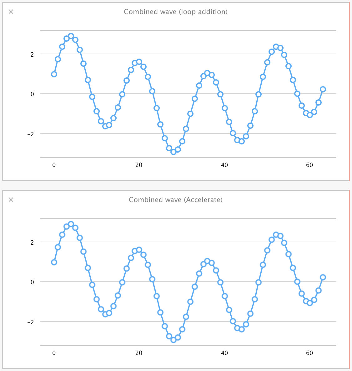
Sure enough, they're the same.
Before moving on to the FFT itself, we will need another vector operation to work on the results from that calculation. All of the values provided from Accelerate's FFT implementation are squares, so we'll need to take their square root. We need to apply a function like sqrt() over each element in that array, so this sounds like another opportunity to use Accelerate.
Accelerate's vecLib library has parallel equivalents of many mathematical functions, including square roots in the form of vvsqrt(). This is a great case for the use of function overloading, so let's create a version of sqrt() that works on arrays of Double values:
								func sqrt(x: [Double]) -> [Double] {
    var results = [Double](count:x.count, repeatedValue:0.0)
    vvsqrt(&results, x, [Int32(x.count)])
    return results
}
Like with our addition operator, this takes in a Double array, creates a blank Double array for output values, and passes those directly into the vvsqrt() Accelerate function. We can verify that this works by typing the following into the playground:
								sqrt(4.0)
sqrt([4.0, 3.0, 16.0])
You'll see that the standard sqrt() function returns 2.0, and our new overload gives back [2.0, 1.73205080756888, 4.0]. In fact, this is such an easy-to-use overload, you can imagine repeating this for all the vecLib functions to create parallel versions of the math functions (and Mattt Thompson has done just that). For a 100000000-element array on a 15" mid-2012 i7 MacBook Pro, our Accelerate-based sqrt() runs nearly twice as fast as a simple array iteration using the normal scalar sqrt().
With that done, let's implement the FFT. We're not going to go into extensive detail on the setup of this, but this is our FFT function:
								let fft_weights: FFTSetupD = vDSP_create_fftsetupD(vDSP_Length(log2(Float(sineArraySize))), FFTRadix(kFFTRadix2))

func fft(var inputArray:[Double]) -> [Double] {
    var fftMagnitudes = [Double](count:inputArray.count, repeatedValue:0.0)
    var zeroArray = [Double](count:inputArray.count, repeatedValue:0.0)
    var splitComplexInput = DSPDoubleSplitComplex(realp: &inputArray, imagp: &zeroArray)

    vDSP_fft_zipD(fft_weights, &splitComplexInput, 1, vDSP_Length(log2(CDouble(inputArray.count))), FFTDirection(FFT_FORWARD));
    vDSP_zvmagsD(&splitComplexInput, 1, &fftMagnitudes, 1, vDSP_Length(inputArray.count));

    let roots = sqrt(fftMagnitudes) // vDSP_zvmagsD returns squares of the FFT magnitudes, so take the root here
    var normalizedValues = [Double](count:inputArray.count, repeatedValue:0.0)

    vDSP_vsmulD(roots, vDSP_Stride(1), [2.0 / Double(inputArray.count)], &normalizedValues, vDSP_Stride(1), vDSP_Length(inputArray.count))
    return normalizedValues
}
As a first step, we set up the FFT weights that need to be used for a calculation of the array size we're working with. These weights are used later on in the actual FFT calculation, but can be calculated via vDSP_create_fftsetupD() and reused for arrays of a given size. Since this array size remains constant in this document, we calculate the weights once as a global variable and reuse them in each FFT.
Within the FFT function, the fftMagnitudes array is initialized with zeroes at the size of our waveform in preparation for it holding the results of the operation. An FFT operation takes complex numbers as input, but we only care about the real part of that, so we initialize splitComplexInput with the input array as the real components, and zeroes for the imaginary components. Then vDSP_fft_zipD() and vDSP_zvmagsD() perform the FFT and load the fftMagnitudes array with squares of the magnitudes from the FFT.
At this point, we use the previously mentioned Accelerate-based array sqrt() operation to take the square root of the squared magnitudes, returning the actual magnitudes, and then normalize the values based on the size of the input array.
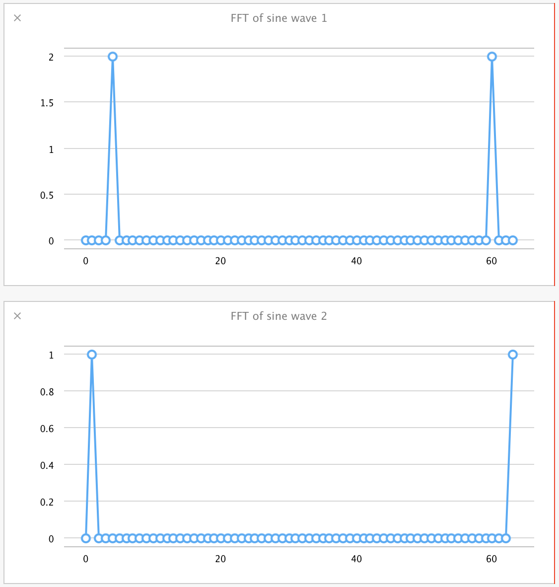
The results from this entire operation look like this for the individual sine waves:
And they look like this for the combined sine wave:
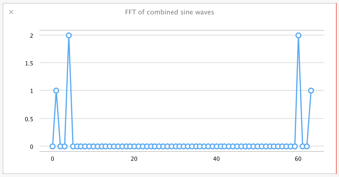
As a very simplified explanation of these values: The results represent 'bins' of sine wave frequencies, starting at the left, with the values in those bins corresponding to the amplitude of the wave detected at that frequency. They are symmetric about the center, so you can ignore the values on the right half of that graph.
What you can observe is that for the frequency 4.0, amplitude 2.0 wave, we see a value of 2.0 binned in bin number 4 in the FFT. Likewise, for the frequency 1.0, amplitude 1.0 wave, we see a 1.0 value in bin number 1 of the FFT. The FFT of the combined sine waves, despite the complex shape of that resultant wave, clearly pulls out the amplitude and frequency of both component waves in their separate bins, as if the FFTs themselves were added.
Again, this is a simplification of the FFT operation, and there are shortcuts taken in the above FFT code, but the point is that we can easily explore even a complex signal processing operation using step-by-step creation of functions in a playground and testing each operation with immediate graphical feedback.
The Case for Rapid Prototyping Using Swift Playgrounds
Hopefully, these examples have demonstrated the utility of Swift playgrounds for experimentation with new libraries and concepts.
At each step in the last case study, we could glance over to the timeline to see graphs of our intermediate arrays as they were processed. That would take a good amount of effort to set up in a sample application and display in an interface of some kind. All of these graphs also update live, so you can go back and tweak a frequency or amplitude value for one of our waveforms and see it ripple through these processing steps. That shortens the development cycle and helps to provide a gut feel for how calculations like this behave.
This kind of interactive development with immediate feedback makes an excellent case for prototyping even complex algorithms in a playground before deployment in a full application.