I'm not sure if this concept is universal, but in North America, the archetypal project for a young and aspiring carpenter is the creation of a dog house; when children become curious about construction and want to fiddle around with hammers, levels, and saws, their parents will instruct them to make one. In many respects, the dog house is a perfect project for the enthusiastic novice. It's grand enough to be inspiring, but humble enough to preclude a sense of crushing defeat if the child happens to screw it up or lose interest halfway through. The dog house is appealing as an introductory project because it is a miniature "Gesamtwerk." It requires design, planning, engineering, and manual craftsmanship. It's easy to tell when the project is complete. When Puddles can overnight in the dog house without becoming cold or wet, the project is a success.

I'm certain that most earnest and curious developers — the kind that set aside their valuable time on evenings and weekends to read a periodical like objc.io — often find themselves in a situation where they're attempting to evaluate tools and understand new and difficult concepts without having an inspiring or meaningful project handy for application. If you're like me, you've probably experienced that peculiar sense of dread that follows the completion of a "Hello World!" tutorial. The jaunty phase of editor configuration and project setup comes to a disheartening climax when you realize that you haven't the foggiest idea what you actually want to make with your new tools. What was previously an unyielding desire to learn Haskell, Swift, or C++ becomes tempered by the utter absence of a compelling project to keep you engaged and motivated.

In this article, I want to propose a "dog house" project for audio signal processing. I'm making an assumption (based on the excellent track record of objc.io) that the other articles in this issue will address your precise technical needs related to Xcode and Core Audio configuration. I'm viewing my role in this issue of objc.io as a platform-agnostic motivator, and a purveyor of fluffy signal processing theory. If you're excited about digital audio processing but haven't a clue where to begin, read on.

Before We Begin

Earlier this year, I authored a 30-part interactive essay on basic signal processing. You can find it here. I humbly suggest that you look it over before reading the rest of this article. It will help to explicate some of the basic terminology and concepts you might find confusing if you have a limited background in digital signal processing. If terms like "Sample," "Aliasing," or "Frequency" are foreign to you, that's totally OK, and this resource will help get you up to speed on the basics.

The Project

As an introductory project to learn audio signal processing, I suggest that you write an application that can track the pitch of a monophonic musical performance in real time .

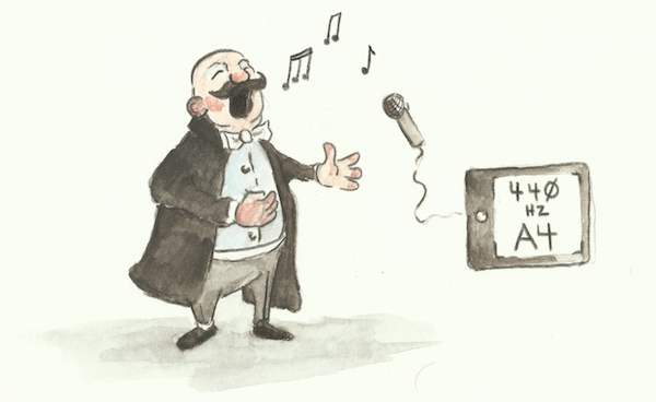
Think of the game "Rock Band" and the algorithm that must exist in order to analyze and evaluate the singing player's vocal performance. This algorithm must listen to the device microphone and automatically compute the frequency at which the player is singing, in real time. Assuming that you have a plump opera singer at hand, we can only hope that the project will end up looking something like this: ¹

I've italicized the word monophonic because it's an important qualifier. A musical performance is monophonic if there is only ever a single note being played at any given time. A melodic line is monophonic. Harmonic and chordal performances are not monophonic, but instead polyphonic. If you're singing, playing the trumpet, blowing on a tin whistle, or tapping on the keyboard of a Minimoog, you are performing a monophonic piece of music. These instruments do not allow for the production of two or more simultaneous notes. If you're playing a piano or guitar, it's quite likely that you are generating a polyphonic audio signal, unless you're taking great pains to ensure that only one string rings out at any given time.

The pitch detection techniques that we will discuss in this article are only suitable for monophonic audio signals. If you're interested in the topic of polyphonic pitch detection, skip to the resources section, where I've linked to some relevant literature. In general, monophonic pitch detection is considered something of a solved problem. Polyphonic pitch detection is still an active and energetic field of research. ²

I will not be providing you with code snippets in this article. Instead, I'll give you some introductory theory on pitch estimation, which should allow you to begin writing and experimenting with your own pitch tracking algorithms. It's easier than you might expect to quickly achieve convincing results! As long as you've got buffers of audio being fed into your application from the microphone or line-in, you should be able to start fiddling around with the algorithms and techniques described in this article immediately.

In the next section, I'll introduce the notion of wave frequency and begin to dig into the problem of pitch detection in earnest.

Sound, Signals, and Frequency

Musical instruments generate sound by rapidly vibrating. As an object vibrates, it generates a longitudinal pressure wave, which radiates into the surrounding air. When this pressure wave reaches your ear, your auditory system will interpret the fluctuations in pressure as a sound. Objects that vibrate regularly and periodically generate sounds which we interpret as tones or notes. Objects that vibrate in a non-regular or random fashion generate atonal or noisy sounds. The most simple tones are described by the sine wave.

This figure visualizes an abstract sinusoidal sound wave. The vertical axis of the figure refers to the amplitude of the wave (intensity of air pressure), and the horizontal axis represents the dimension of time. This sort of visualization is usually called a waveform drawing, and it allows us to understand how the amplitude and frequency of the wave changes over time. The taller the waveform, the louder the sound. The more tightly packed the peaks and troughs, the higher the frequency.

The frequency of any wave is measured in hertz. One hertz is defined as one cycle per second. A cycle is the smallest repetitive section of a waveform. If we knew that the width of the horizontal axis corresponded to a duration of one second, we could compute the frequency of this wave in hertz by simply counting the number of visible wave cycles.

In the figure above, I've highlighted a single cycle of our sine wave using a transparent box. When we count the number of cycles that are completed by this waveform in one second, it becomes clear that the frequency of the wave is exactly 4 hertz, or four cycles per second. The wave below completes eight cycles per second, and therefore has a frequency of 8 hertz.

Before proceeding any further, we need some clarity around two terms I have been using interchangeably up to this point. Pitch is an auditory sensation related to the human perception of sound. Frequency is a physical, measurable property of a waveform. We relate the two concepts by noting that the pitch of a signal is very closely related to its frequency. For simple sinusoids, the pitch and frequency are more or less equivalent. For more complex waveforms, the pitch corresponds to the fundamental frequency of the waveform (more on this later). Conflating the two concepts can get you into trouble. For example, given two sounds with the same fundamental frequency, humans will often perceive the louder sound to be higher in pitch. For the rest of this article, I will be sloppy and use the two terms interchangeably. If you find this topic interesting, continue your extracurricular studies here.

Pitch Detection

Stated simply, algorithmic pitch detection is the task of automatically computing the frequency of some arbitrary waveform. In essence, this all boils down to being able to robustly identify a single cycle within a given waveform. This is an exceptionally easy task for humans, but a difficult task for machines. The CAPTCHA mechanism works precisely because it's quite difficult to write algorithms that are capable of robustly identifying structure and patterns within arbitrary sets of sample data. I personally have no problem picking out the repeating pattern in a waveform using my eyeballs, and I'm sure you don't either. The trick is to figure out how we might program a computer to do the same thing quickly, in a real-time, performance-critical environment. ³

The Zero-Crossing Method

As a starting point for algorithmic frequency detection, we might notice that any sine wave will cross the horizontal axis two times per cycle. If we count the number of zero-crossings that occur over a given time period, and then divide that number by two, we should be able to easily compute the number of cycles present within a waveform. For example, in the figure below, we count eight zero-crossings over the duration of one second. This implies that there are four cycles present in the wave, and we can therefore deduce that the frequency of the signal is 4 hertz.

We might begin to notice some problems with this approach when fractional numbers of cycles are present in the signal under analysis. For example, if the frequency of our waveform increases slightly, we will now count nine zero-crossings over the duration of our one-second window. This will lead us to incorrectly deduce that the frequency of the purple wave is 4.5 hertz, when it's really more like 4.6 hertz.

We can alleviate this problem a bit by adjusting the size of our analysis window, performing some clever averaging, or introducing heuristics that remember the position of zero-crossings in previous windows and predict the position of future zero-crossings. I'd recommend playing around a bit with improvements to the naive counting approach until you feel comfortable working with a buffer full of audio samples. If you need some test audio to feed into your iOS device, you can load up the sine generator at the bottom of this page.

While the zero-crossing approach might be workable for very simple signals, it will fail in more distressing ways for complex signals. As an example, take the signal depicted below. This wave still completes one cycle every 0.25 seconds, but the number of zero-crossings per cycle is considerably higher than what we saw for the sine wave. The signal produces six zero-crossings per cycle, even though the fundamental frequency of the signal is still 4 hertz.

While the zero-crossing approach isn't really ideal for use as a hyper-precise pitch tracking algorithm, it can still be incredibly useful as a quick and dirty way to roughly measure the amount of noise present in a signal. The zero-crossing approach is appropriate in this context because noisy signals will produce more zero-crossings per unit time than cleaner, more tonal sounds. Zero-crossing counting is often used in voice recognition software to distinguish between voiced and unvoiced segments of speech. Roughly speaking, voiced speech usually consists of vowels, where unvoiced speech is produced by consonants. However, some consonants, like the English "Z," are voiced (think of saying "zeeeeee").

Before we move on to introducing a more robust approach to pitch detection, we first must understand what is meant by the term I bandied about in earlier sections. Namely, the fundamental frequency.

The Fundamental Frequency

Most natural sounds and waveforms are not pure sinusoids, but amalgamations of multiple sine waves. While Fourier Theory is beyond the scope of this article, you must accept the fact that physical sounds are (modeled by) summations of many sinusoids, and each constituent sinusoid may differ in frequency and amplitude. When our algorithm is fed this sort of compound waveform, it must determine which sinusoid is acting as the fundamental or foundational component of the sound and compute the frequency of that wave.

I like to think of sounds as compositions of spinning, circular forms. A sine wave can be described by a spinning circle, and more complex wave shapes can be created by chaining or summing together additional spinning circles. ⁴ Experiment with the visualization below by clicking on each of the four buttons to see how various compound waveforms can be composed using many individual sinusoids.

The blue spinning circle at the center of the diagram represents the fundamental, and the additional orbiting circles describe overtones of the fundamental. It's important to notice that one rotation of the blue circle corresponds precisely to one cycle in the generated waveform. In other words, every full rotation of the fundamental generates a single cycle in the resulting waveform. ⁵

I've again highlighted a single cycle of each waveform using a grey box, and I'd encourage you to notice that the fundamental frequency of all four waveforms is identical. Each has a fundamental frequency of 4 hertz. Even though there are multiple sinusoids present in the square, saw, and wobble waveforms, the fundamental frequency of the four waveforms is always tied to the blue sinusoidal component. The blue component acts as the foundation of the signal.

It's also very important to notice that the fundamental is not necessarily the largest or loudest component of a signal. If you take another look at the "wobble" waveform, you'll notice that the second overtone (orange circle) is actually the largest component of the signal. In spite of this rather dominant overtone, the fundamental frequency is still unchanged. ⁶

In the next section, we'll revisit some university math, and then investigate another approach for fundamental frequency estimation that should be capable of dealing with these pesky compound waveforms.

The Dot Product and Correlation

The dot product is probably the most commonly performed operation in audio signal processing. The dot product of two signals is easily defined in pseudo-code using a simple for loop. Given two signals (arrays) of equal length, their dot product can be expressed as follows:

								func dotProduct(signalA: [Float], signalB: [Float]) -> [Float] {
    return map(zip(signalA, signalB), *)
}

							

Hidden in this rather pedestrian code snippet is a truly wonderful property. The dot product can be used to compute the similarity or correlation between two signals. If the dot product of two signals resolves to a large value, you know that the two signals are positively correlated. If the dot product of two signals is zero, you know that the two signals are decorrelated — they are not similar. As always, it's best to scrutinize such a claim visually, and I'd like you to spend some time studying the figure below.

Shift

This visualization depicts the computation of the dot product of two different signals. On the topmost row, you will find a depiction of a square wave, which we'll call Signal A. On the second row, there is a sinusoidal waveform we'll refer to as Signal B. The waveform drawn on the bottommost row depicts the product of these two signals. This signal is generated by multiplying each point in Signal A with its vertically aligned counterpart in Signal B. At the very bottom of the visualization, we're displaying the final value of the dot product. The magnitude of the dot product corresponds to the integral, or the area underneath this third curve.

As you play with the slider at the bottom of the visualization, notice that the absolute value of the dot product will be larger when the two signals are correlated (tending to move up and down together), and smaller when the two signals are out of phase or moving in opposite directions. The more that Signal A behaves like Signal B, the larger the resulting dot product. Amazingly, the dot product allows us to easily compute the similarity between two signals.

In the next section, we'll apply the dot product in a clever way to identify cycles within our waveforms and devise a simple method for determining the fundamental frequency of a compound waveform.

Autocorrelation

The autocorrelation is like an auto portrait, or an autobiography. It's the correlation of a signal with itself. We compute the autocorrelation by computing the dot product of a signal with a copy of itself at various shifts or time lags. Let's assume that we have a compound signal that looks something like the waveform shown in the figure below.

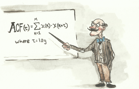
We compute the autocorrelation by making a copy of the signal and repeatedly shifting it alongside the original. For each shift (lag), we compute the dot product of the two signals and record this value into our autocorrelation function. The autocorrelation function is plotted on the third row of the following figure. For each possible lag, the height of the autocorrelation function tells us how much similarity there is between the original signal and its copy.

Lag: -60

Slowly move the slider at the bottom of this figure to the right to explore the values of the autocorrelation function for various lags. I'd like you to pay particular attention to the position of the peaks (local maxima) in the autocorrelation function. For example, notice that the highest peak in the autocorrelation will always occur when there is no lag. Intuitively, this should make sense because a signal will always be maximally correlated with itself. More importantly, however, we should notice that the secondary peaks in the autocorrelation function occur when the signal is shifted by a multiple of one cycle. In other words, we get peaks in the autocorrelation every time that the copy is shifted or lagged by one full cycle, since it once again "lines up" with itself.

The trick behind this approach is to determine the distance between consecutive prominent peaks in the autocorrelation function. This distance will correspond precisely to the length of one waveform cycle. The longer the distance between peaks, the longer the wave cycle and the lower the frequency. The shorter the distance between peaks, the shorter the wave cycle and the higher the frequency. For our waveform, we can see that the distance between prominent peaks is 0.25 seconds. This means that our signal completes four cycles per second, and the fundamental frequency is 4 hertz — just as we expected from our earlier visual inspection.

The autocorrelation is a nifty signal processing trick for pitch estimation, but it has its drawbacks. One obvious problem is that the autocorrelation function tapers off at its left and right edges. The tapering is caused by fewer non-zero samples being used in the calculation of the dot product for extreme lag values. Samples that lie outside the original waveform are simply considered to be zero, causing the overall magnitude of the dot product to be attenuated. This effect is known as biasing , and can be addressed in a number of ways. In his excellent paper, "A Smarter Way to Find Pitch," Philip McLeod devises a strategy that cleverly removes this biasing from the autocorrelation function in a non-obvious but very robust way. When you've played around a bit with a simple implementation of the autocorrelation, I would suggest reading through this paper to see how the basic method can be refined and improved.

Autocorrelation as implemented in its naive form is an O(N ² ) operation. This complexity class is less than desirable for an algorithm that we intend to run in real time. Thankfully, there is an efficient way to compute the autocorrelation in O(N log(N)) time. The theoretical justification for this algorithmic shortcut is far beyond the scope of this article, but if you're interested, you should know that it's possible to compute the autocorrelation function using two FFT (Fast Fourier Transform) operations. You can read more about this technique in the footnotes. ⁷ I would suggest writing the naive version first, and using this implementation as a ground truth to verify a fancier, FFT-based implementation.

Latency and the Waiting Game

Real-time audio applications partition time into chunks or buffers. In the case of iOS and OS X development, Core Audio will deliver buffers of audio to your application from an input source like a microphone or input jack and expect you to regularly provide a buffer's worth of audio in the rendering callback. It may seem trivial, but it's important to understand the relationship of your application's audio buffer size to the sort of audio material you want to consider in your analysis algorithms.

Let's walk through a simple thought experiment. Pretend that your application is operating at a sampling rate of 128 hertz, ⁸ and your application is being delivered buffers of 32 samples. If you want to be able to detect fundamental frequencies as low as 2 hertz, it will be necessary to collect two buffers worth of input samples before you've captured a whole cycle of a 2 hertz input wave.

The pitch detection techniques discussed in this article actually need two or more cycles worth of input signal to be able to robustly detect a pitch. For our imaginary application, this means that we'd have to wait for two more buffers of audio to be delivered to our audio input callback before being able to accurately report a pitch for this waveform.

This may seem like stating the obvious, but it's a very important point. A classic mistake when writing audio analysis algorithms is to create an implementation that works well for high-frequency signals, but performs poorly on low-frequency signals. This can occur for many reasons, but it's often caused by not working with a large enough analysis window — by not waiting to collect enough samples before performing your analysis. High-frequency signals are less likely to reveal this sort of problem because there are usually enough samples present in a single audio buffer to fully describe many cycles of a high-frequency input waveform.

The best way to handle this situation is to push every incoming audio buffer into a secondary circular buffer. This circular buffer should be large enough to accommodate at least two full cycles of the lowest pitch you want to detect. Avoid the temptation to simply increase the buffer size of your application. This will cause the overall latency of your application to increase, even though you only require a larger buffer for particular analysis tasks.

You can reduce latency by choosing to exclude very bassy frequencies from your detectable range. For example, you'll probably be operating at a sample rate of 44,100 hertz in your OS X or iOS project, and if you want to detect pitches beneath 60 hertz, you'll need to collect at least 2,048 samples before performing the autocorrelation operation. If you don't care about pitches beneath 60 hertz, you can get away with an analysis buffer size of 1,024 samples.

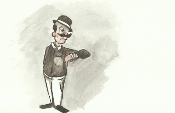
The important takeaway from this section is that it's impossible to instantly detect pitch. There's an inherent latency in any pitch tracking approach, and you must simply be willing to wait. The lower the frequencies you want to detect, the longer you'll have to wait. This tradeoff between frequency coverage and algorithmic latency is actually related to the Heisenberg Uncertainty Principle, and permeates all of signal processing theory. In general, the more you know about a signal's frequency content, the less you know about its placement in time.

References and Further Reading

I hope that by now you have a sturdy enough theoretical toehold on the problem of fundamental frequency estimation to begin writing your own monophonic pitch tracker. Working from the cursory explanations in this article, you should be able to implement a simple monophonic pitch tracker and dig into some of the relevant academic literature with confidence. If not, I hope that you at least got a small taste for audio signal processing theory and enjoyed the visualizations and illustrations.

The approaches to pitch detection outlined in this article have been explored and refined to a great degree of finish by the academic signal processing community over the past few decades. In this article, we've only scratched the surface, and I suggest that you refine your initial implementations and explorations by digging deeper into two exceptional examples of monophonic pitch detectors: the SNAC and YIN algorithms.

Philip McLeod's SNAC pitch detection algorithm is a clever refinement of the autocorrelation method introduced in this article. McLeod has found a way to work around the inherent biasing of the autocorrelation function. His method is performant and robust. I highly recommend reading McLeod's paper titled "A Smarter Way to Find Pitch" if you want to learn more about monophonic pitch detection. It's one of the most approachable papers on the subject. There is also a wonderful tutorial and evaluation of McLeod's method available here . I highly recommend poking around this author's website.

YIN was developed by Cheveigné and Kawahahara in the early 2000s, and remains a classic pitch estimation technique. It's often taught in graduate courses on audio signal processing. I'd definitely recommend reading the original paper if you find the topic of pitch estimation interesting. Implementing your own version of YIN is a fun weekend task.

If you're interested in more advanced techniques for polyphonic fundamental frequency estimation, I suggest that you begin by reading Anssi Klapuri's excellent Ph.D. thesis on automatic music transcription. In his paper, he outlines a number of approaches to multiple fundamental frequency estimation, and gives a great overview of the entire automatic music transcription landscape.

If you're feeling inspired enough to start on your own dog house, feel free to contact me on Twitter with any questions, complaints, or comments about the content of this article. Happy building!